1. Introduction

Time varying parameter models have a long history in statistics. Modelling unequal variances in nonlinear time series is a challenging task. The ideas and techniques of modelling time series in these diverse areas of science and other related disciplines are proved to be useful and innovative by Box and Jenkins[4], Engle[9], Gilks and Berzuini[16] and[30]. Bilinear Generalized Autoregressive Conditional Heteroskedasticity (BL-GARCH) model is one of the major tools that Economists use to model financial markets’ behaviour in the presence of political disorders, economic crises, wars or natural disasters. In such stress periods, prices of financial assets tend to fluctuate very profusely[30].

Statistically speaking, if the conditional variance of given that is, of a time series is not constant over time then the process is conditionally heteroskedastic. Heteroskedasticity refers to the random errors having unequal variances. In particular, a heteroskedastic model has , Christensen[7]. Let ) be a Gaussian vector with mean vector and variance matrix

If the expected value of all error terms when squared is the same at any given point, then the vector is homogeneous (homoskedastic) that is, When this assumption does not hold, the vector is heteroskedastic, see Box, Jenkins and Reinsel[5], Bollerslev, Engle and Nelson[3]. There are several approaches to dealing with heteroskedasticity. If the error variance at different times is known, weighted regression is a good method. If as is the case with financial time series, the error variance is unknown, and must be estimated from the data, we can model the changing error variance with the bilinear generalized autoregressive conditional heteroskedasticity model.

2. Literature Review

In the past decades, many researchers have introduced informal and ad-hoc procedures to take account of the changes in the variance. One of the first authors to address variance changing over time was Mandelbrot (1963), who used recursive estimates of the variance for modelling volatility. Klein (1977) used rolling estimates of quadratic residuals.

Engle (1982) proposes Autoregressive Conditional Heteroskedasticity (ARCH (q)) models that seem to capture the empirical characteristics in the financial time series. The models have non-constant variances conditioned on the past, which is a linear aggregate of recent past disturbances. This means that the more recent news will be the fundamental information that is relevant for modelling the present volatility. Some leading scholars who studied ARCH models include: Geweke[14, 15], Diebold and Nerlove (1989), Engle[10], Jones, Kaul and Lipson[19] and Gourieroux[17]. Harvey, Ruiz and Sentana (1992) established the existence of a few common factors explaining exchange rate volatility movements. Engle, Ng and Rothschild[11] show that U. S. bond volatility changes are closely linked across maturities. This commonality of volatility changes holds not only across assets within a market, but also across different markets. For example, Schwert[31] established that U. S. stock and bond volatilities move together, while Engle and Susmel[12], Hamao, Masulia and Ng[18] discovered close links between volatility changes across international stock markets. Lamoureux and Lastrapes[21] deduced that conditional heteroskedasticity may be caused by time dependence in the rate of information arrival to the market. They use the daily trading volume of stock markets as a proxy for such information arrival and confirm its significance. Mizrach[25] associates ARCH models with the errors of the economic agent’s learning processes. Cai[6] proposed the switching ARCH or SWARCH model in which there are several different ARCH models and that the economy switches from one to another following a Markov chain. In this model there can be extremely high volatility process which is responsible for events such as the stock market crash in 2009. That volatilities move together should be encouraging to model builders, since it indicates that a few common factors may explain much of the temporal variation in the conditional variances and covariances of asset returns.

Storti and Vitale[32] proposed BL-GARCH model in Gaussian framework. Diongue, Guegan and Wolff[9] extended their works using elliptical noise to capture the leverage effect or negative correlation between asset returns and volatility.

3. Methodology

The paper adapts recommended three iterative steps of Box-Jenkins to select a suitable stochastic model, Box and Jenkins (4), Box, Jenkins and Reinsel[5]. The steps are

(i) Identification

(ii) Estimation

(iii) Diagnostic Checks

The aim of the identification stage is to determine the transformation required to produce stationarity and also the order of AR and MA operators for the series. In a typical BL-GARCH modelling application, it is preferable that there are a minimum of about 80 data points in the series in order to get reasonable MLEs for the parameters. This identification starts with time series plot which may reveal one of the following characteristics:

(i) trends either in the mean level or variance of the time series

(ii) extreme values and outliers

(iii) seasonality

At the estimation stage, estimates are usually calculated for the conditional mean, ARCH, GARCH and leverage effect parameters using Maximum Likelihood Estimates (MLE). In this paper, natural logarithms are applied to obtain the transformation required to produce stationarity. The normality assumption of the residuals is usually not critical for obtaining good parameter estimates. As long as the ’s are independent and possess finite variance, reasonable estimates (Gaussian estimates) of the parameters can be obtained, Abass[1], Onyeka-Ubaka, Abass and Okafor[27]. Having observed that the conditional variance depends on the data, the paper adapted maximum likelihood method which is consistent and asymptotically normal. This is because financial time series data, for which BL-GARCH models are usually capable of capturing the characteristics, generate high frequency sampling of data.

The paper uses the Gaussian (Normal) and the non-Gaussian (Generalized Student t) distributions to allow the model fit both the tails and the central part of the conditional distribution present in high frequency financial time series data. The elliptical normalized distributions: the Normal and the Generalized Student t considered in this paper belong to exponential class. This is because their distributions can be expressed as

This implies that they have complete sufficient statistics for the estimators. (a) The normal distribution is uniquely determined by its first two moments (Dallah, Okafor and Abass[8]). Hence, only the conditional mean and variance parameters enter the log-likelihood function

(1)

where n is the sample size.

To obtain an analytical or numerical solution of the MLE, it is necessary to obtain the first derivative and solve . Assuming , we have the score functions as

(2)

Now, if the paper assumes that the innovations have a conditional non-Gaussian:

(b) The Student t distribution is given as

(3)

(c) The Generalized Student t distribution is given as

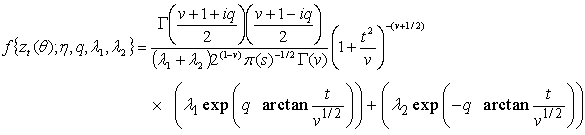(4)

where , q is a complex number. . and are the left and right tail parameter respectively, v is the degrees of freedom. The standardized deviate has distribution t(0, 1, v), where x is the observations, is the mean and s is the standard deviation of the observations.

Note: is a necessary condition because the probability density function must always be positive. Also the normalization constant

of (4) is real, because the integrand is a real function on . It is clear that if q = 0 in (4), the usual Student t distribution is derived. Moreover, for q = 0, the normalization constant of distribution (4) is equal to the normalization constant of Student t distribution. The kurtosis of the Student t distribution is

which is greater than three if v < 4.

The MLE estimator maximizes the log-likelihood function given by

(5)

where and is the Euler gamma function defined by . When , we have the normal distribution, so that the smaller the value of v the fatter the tails.

This means that for large v, the product

tends to unity, while the right-hand bracket in (3) tends to .

The score function is given by

(6)

and the Hessian matrix is given by

(7)

4. Results and Discussion

In this paper, a BL-GARCH model is introduced in which the innovation is composed of several sources of errors where each of the error sources has heteroskedastic specifications of the GARCH form. Since the error components cannot be separately observed given past observations, the independent variables in the variance equations are not measurable with respect to the available information set, which complicates procedures. Following earlier work of 2and Vitale[31] and adapting Mohler[26] nonlinear representation of bilinear model, the state space representation of a bilinear model (of order m) in the control theory literatures is of the general form

(10)

where the system matrix A and the input matrix B are square matrices of order the state vector x and the control vector are column vectors of order . The input is a usually unobservable random process and the systems coefficient matrices are to be estimated.

If the paper nests the GARCH model and (10), the BL-GARCH model is given as

(11)

(12)

(13)

Given the parameter space, , and the expected parameter vector, , the assumption is that the parameter is in the interior of , a compact parameter space.

Specifically, for any vector , we assume that

(a) The AR and MA polynomials have no common roots and that all their roots lie outside the unit circle.

(b) and

(c) , for

(d)

where the compact space is given as

The generalized student t distribution with one skewness parameter and two tail parameters offers the study the potential to improve our ability to fit the data in the tail regions which are critical to the risk management and other financial economic application. This is because downward movement of the markets is followed by higher volatilities than upward movement of the same magnitude, see Pagan and Schwert[29], Locke and Sayers (1993), Linton[22], Muller and Yohai (2002), Eraker, Johannes and Polson[13]. So it is important to use BL-GARCH (1, 1) model to capture asymmetric shocks to volatility. This distribution function will be acceptable if it converges to the probability density of the standard normal distribution.

Proposition 4.1

If as in (4) is distribution flexible, then it contains Pearson subordinate distributions.

Proof

The generalized student t distribution can be derived from a generalization of the Pearson differential equation as follows

(14)

where g(z) and h(z) are polynomials in the random variable z, and f(z) is the density function of z. In the standard Pearson system, g(z) is a polynomial in z of the degree less than or equal to one, whereas h(z) is a polynomial in z of degree less than or equal to two. The generalized solution of (14) is

(15)

where the normalizing constant is given by

(16)

The domain D of f(z) in (16) is the open interval where h(z) is positive.

The choice of and for the generalized student t distribution are

(17)

(18)

By substituting (17) and (18) in (14), the generalized student t distribution is given by

(19)

where

(20)

And the distribution parameters are functions of the parameters

given in (17) and (18). Provided that in (19), , all moments of the distribution exist. This distribution can exhibit a range of shapes including fat tails; sharp peaks and even multimodality (see Lye et al (1998)).

As the generalized student t distribution given by (20) is derived from an extension of the Pearson exponential family, it directly contains many of the Pearson subordinate distributions as special cases. In particular, from the point of view of the existing ARCH models, these special cases include the Normal and Student t distributions. The standard normal distribution occurs when and all remaining parameters are zero. The Student t distribution occurs when and all remaining parameters are zero.

A special case which turns out to be important in the empirical application is given by (20) with and .

(21)

where is the normalized constant. This distribution is referred to as the skewed Student t distribution where skewness is controlled by the parameter, . When, there is no skewness and the distribution becomes Student t distribution.

This completes the proof.

4.1. Empirical Study of Real Data

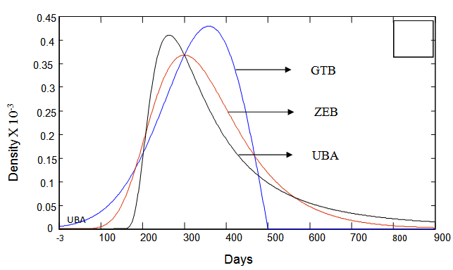
Four banks: First Bank of Nigeria (FBN), Guaranty Trust Bank (GTB), United Bank for Africa (UBA) and Zenith Bank (ZEB) were selected for the study by means of purposive sampling technique. These four banks were selected because they are considered to be more susceptible to volatility than other banks and had passed the screening exercise conducted by Central Bank of Nigeria (CBN) in August, 2009. Their volume of stocks traded on the floor of the Nigeria Stock Exchange (NSE) for the sample period were collected and analyzed using BL-GARCH model to observe the volatile nature of stocks within the sampled period. The series plots of the banks that exhibited heavier tails are shown below.

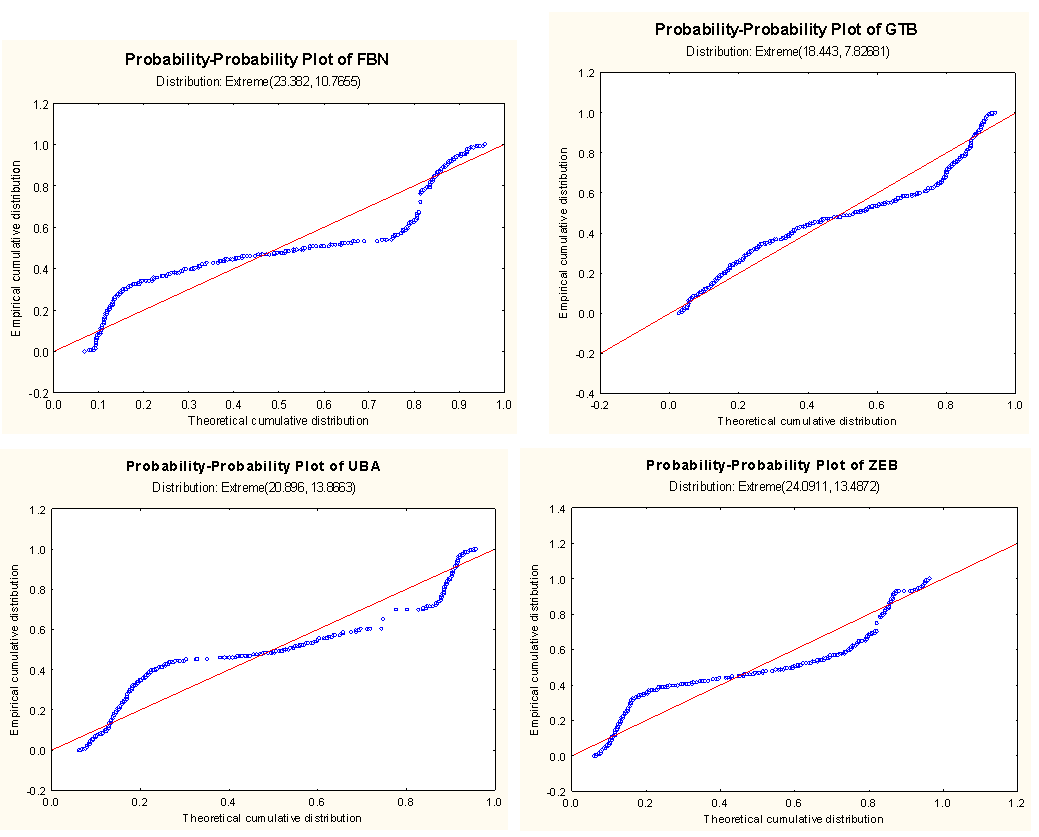
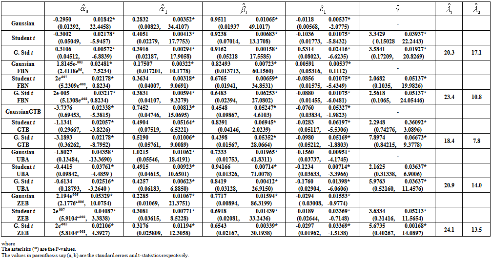
Figure 1 shows that the generalized student t distribution seems to be a more appropriate distribution for the selected banks data. The generalized student t distribution allows for situations where the tails are heavier or lighter than the usual student t distribution. The extreme values (left and right tails) for different banks are estimated automatically together with the plot of the P-P plot of the selected banks in Figure 2.

The probability-probability plots of the four banks show that they are primarily a few large outliers that cause the departures of the system from normality as obtainable from Figure 2. These departures are pointing out that there are other factors that interrupt the expected volatility of stock market prices of these banks on the floor of the Nigeria Stock Exchange. The factors may include among other things, giving loans to private and corporate firms to buy shares without due process, lack of strategic management and regular supervision. If the residuals are normally distributed, the P-P plot should lie on a straight line.

The parameter results estimated by methods of the Maximum Likelihood Estimator (MLE) using MATLAB (R2008b) soft ware were given in Table 1.

Table 1 represents conditional variance BL-GARCH (1, 1) model parameter estimation results. Results reveal that parameter estimates are satisfactory (asymptotically unbiased, efficient and consistent) in that the standard errors are small and the t-statistic for GARCH parameters is high. It is clear from the analysis that estimate and in the BL-GARCH (1, 1) model are significant at the 5% level with the volatility coefficient greater in magnitude. Hence, the hypothesis of constant variance is rejected, at least within sample. Furthermore, the stationarity condition is satisfied for the three distributions, as at the maximum of the respective log-likelihood functions. Even when , so long as , covariance stationarity is established. The estimated asymmetric volatility response is negative and significant for all models confirming the usual expectation in stock markets where downward movements (falling returns) are followed by higher volatility than upward movements (increasing returns). The results also follow the empirical findings of Storti and Vitale[32], in that the kurtosis strongly depends on the leverage-effect response parameter. The results indicate that the BL-GARCH (1, 1) processes are appropriate for modelling the conditional variance of the selected banks return. Using Akaike (1974), the BL-GARCH (1, 1) model with minimum AIC was selected as the best.

The BL-GARCH (1, 1) conditional variance model that best fits the observed data is

Figure 1. Plots of Generalized Student t Distribution for Banks that exhibit Heavier and Lighter Tails

Figure 2. Probability-Probability (P-P) Plots with Extreme Values for the Four Banks

Table 1. Conditional Variance BL-GARCH (1, 1) Model Parameter Estimation Results

where

From the results obtained, the BL-GARCH (1, 1) model with Generalized Student t distribution fits GTB, UBA and ZEB data better while the First Bank of Nigeria data follows the Student t BL-GARCH (1, 1) models. This is because adding more parameters in modelling the FBN data does not improve the parameter estimates of the FBN. The parameteris therefore a good approximation of the degree up to which one is able to explain the variance/kurtosis of the disturbances. The GTB, UBA and ZEB series confirm these statements as seen in Figure 1.

5. Conclusions

The newly introduced generalized student t distribution in this paper is the most general of all the useful distributions applied in the BL-GARCH model parameter estimation. It offers a three parameter form which makes it more general than those available in the literature for obtaining empirical characteristics such as volatility clustering, leptokurtosis and leverage effect between returns and conditional variances as well as capturing heavier and lighter tails in high frequency financial time series data. The results of the extreme departure of some data are very crucial to risk managers in planning and decision making processes. Thus, the empirical results of BL-GARCH model show that parameters can be evaluated from Gaussian and non-Gaussian distributions.