1. Introduction

The importance of nutrition on early-childhood development outcomes has gained international awareness. Strong evidence shows that nutritional failure during pregnancy and in the first two years of life lead to lower human capital endowments, negatively affecting physical strength and cognitive ability in adults. This contributes directly reduced earnings potential of individuals and damages national economic growth and competitiveness potential in a globalized world[1].

Undernutrition of children is among the most serious health issues facing developing countries. Malnutrition is particularly prevalent in developing countries, where it affects one out of every three pre-school age children. It is an intrinsic indicator of well-being, but is also associated with morbidity, mortality, impaired childhood development, and reduced labor productivity[2]. Reducing malnutrition rates by half is one of the central development goals adopted by the international community at the Millennium Summit[3]. Malnutrition is an underlying factor in many diseases in both children and adults, and it contributes greatly to the disability - adjusted life years worldwide.

Nutrition and health are important dimensions of human well-being. Undernutrition may be defined as insufficient intake of energy and nutrients to meet an individual’s needs to maintain good health. Additionally, it may indicate insufficient absorption of nutrients due to ill health. The term “malnutrition” is sometimes also used synonymously for Undernutrition. However, strictly speaking, malnutrition includes both Undernutrition as well as over-nutrition. Over nutrition simply refers to excess intake of macronutrients and micronutrients[4]. In the developing world, it is the Undernutrition which is of greater concern because it is alleged to be one of the leading causes of morbidity in children and contributes to more than half of child deaths[5]. Nutritional deprivation in early life can have long lasting effects on growth, educational attainment and productivity. Usually, the under-nutrition in children (under age five) is used as a measure for determining the extent of this particular public health problem in a population[6, 7].

The development of Undernutrition typically follows a pattern that is closely related to the age of the child. While some children are already born undernourished due to growth retardation in utero, the anthropometric status of children worsens considerably only after 4-6 months, when children are weaned and solid foods are introduced 6,8]. Initially, the worsening anthropometric status shows up as acute under-nutrition. But then stunting develops and worsens until about age 2-3. At that time, the body has, through reduced growth, adjusted to reduced nutritional intake and now needs fewer nutrients to maintain this smaller[6,9].

Nutritional status during childhood has consequences in childhood until adulthood. Deficiencies in nutrients or imbalances between them can have dire long-term effects for the individual[10]. Thus, measuring the child’s nutritional status is important because of both the long-term and short-term effects on the health, educational and the cognitive abilities of the child. There are also severe consequences and effects to the child’s ability to function as a healthy, productive and self-supporting community member in the long-term, which is another reason for concern, and as such the study further wishes to add to an understanding on how to contribute to the betterment of society.

Measures of child malnutrition are based on height-for-age, weight-for-age, and weight-for-height. Each of these indices provides somewhat different information about the nutritional status of child. The height-for-age index measures linear growth retardation among children, primarily reflecting chronic malnutrition. The weight – for - height index measures body mass in relation to body height, primarily reflecting acute malnutrition. Weight-for-age reflects both chronic and acute malnutrition[6, 4].

According to the 2009, special report of the Crop and Food Security Assessment Mission to Ethiopia[11], 7.5 million persons are still chronically food insecure and are under the productive safety net programme (PSNP); an additional 4.9 million people are facing acute food insecurity as of January to June 2009. Malnutrition in Ethiopia is the underlying cause of 57% of child deaths and thus failing to address this problem will also hold back progress towards reaching MDG 4 to reduce child mortality[12].

Woldemariam and Timotiows (2002) performed a comparative study for urban, rural and combined urban and rural children. They identified region of residence, education of mother, economic status of the household and age of the child as determinants of malnutrition and health problems among urban children. For rural children, the analyses showed that region of residence, education of mother, education of partner, age, birth order and preceding birth interval of a child as important predictors of nutrition status. The combined urban and rural (national) sample results indicated that region of residence, education of mother, education of father, economic status of the household, age, birth order and birth interval of the child were important determinants of child nutrition and health status.[13]

Nutritional status of children in Ethiopia is among the worst in the world. For example, chronic malnutrition in Ethiopia is worst than other SSA countries: about one in two children (51 percent) are moderately to severely stunted, of which slightly more than one in four children (26 percent) are severely stunted . Thus, high malnutrition rates in Ethiopia pose a significant obstacle to achieve better child health outcomes[12].

The implication of this high prevalence of child malnutrition is that a good knowledge regarding the major factors that contribute to the problem is essential in order to avoid its adverse consequences. The causes and determinants of child malnutrition are complex, interrelated, and multidimensional. In the literature, since mothers are the main providers of primary care to their children, understanding the contribution of maternal characteristics on child nutrition has been identified as a key towards addressing the problem of child malnutrition. In Ethiopia reason behind malnutrition is still to be known from recent data available.

Weight-for-age was chosen as the index of child nutritional status for this analysis because it is the most widely used in developing countries, allowing for the inclusion of the largest number of studies. Although it does not distinguish between wasting and stunting, low weight-for-age (underweight) represents a combination of both aspects and has a high positive predictive value as an indicator for child malnutrition in developing countries[6].

While there are numerous studies on childhood malnutrition in Ethiopia and other countries, majority of these studies have looked at the contributions of individual ‐ level (socioeconomic and family planning) characteristics. A growing body of literature considers the importance of understanding of determinants of childhood malnutrition through an integrated analysis that considers linkages between demographic, household, and community structures. Thus, the contextual aspect of child malnutrition needs to be explored to understand the process of malnourishment as a whole. The study was to model the various possible factors and their contribution for the current high prevalence of malnutrition problems using the Bayesian semi-parametric regression model. To expand our understanding of the most common and consistent factors on the risk of childhood malnutrition, it is necessary to consider expected determinants for malnutrition using Bayesian approach. Therefore, the purpose of this paper has been to develop and test a model for childhood nutritional status.

2. Data and Methodology

2.1. Data

This research used the 2011 Ethiopian Demographic and Health Survey. The survey drew a representative sample of women of reproductive age, by administering a questionnaire and making an anthropometric assessment of women and their children that were born within the previous five years.

For the 2011 EDHS, a representative sample of approximately 17,817 households from 624 clusters was selected. In the first stage, 624 clusters, 187 urban and 437 rural were selected from the list of enumeration areas based on sampling frame. In the second stage, a complete listing of households was carried out in each selected cluster. The analysis presented in this study on nutritional status was based on the 8200 children aged less than 60 months with complete anthropometric measurements.

In this study, height and weight measurements of the children, taking age and sex into consideration, were converted into Z‐scores based on new growth standards published by the World Health Organization (WHO) in 2006. Thus, those below (-2) standard deviations of the WHO median reference for height‐for‐age, weight‐for‐age and weight‐for‐height were defined as stunted, underweight, and wasted, respectively. In this study, underweight was considered as an indicator of both linear growth retardation and acute malnutrition. Children with weight‐for‐age z‐scores below two standard deviations from the median of the reference population were considered as underweight. Furthermore, children with z‐scores below (-3) standard deviations from the median of the reference population were considered to be severely underweight, while children with z‐scores between three and two standard deviations were considered to be moderately underweight; these all three indicators are used to describe the level of child malnutrition and the relationship between maternal and child nutritional status. Moreover, underweight measures linear growth retardation, cumulative growth deficit and acute malnutrition and indicates the effect of chronic and acute nutritional status in the life of the child. Therefore, an in‐depth analysis was performed on underweight by focusing on factors affecting chronic and acute malnutrition.

Undernutrition among children is usually determined by assessing the anthropometric status of a child relative to a reference standard. In this study, under-nutrition was considered as measured by underweight or insufficient weight‐for‐age, indicating chronic and acute under-nutrition. Weight‐for‐age score for a child i is determined using a Z‐score which is defined as

where AI refers to the child`s anthropometric indicator (weight at a certain age in our case), MAI refers to the median of the reference population and σ refers to the standard deviation of the reference population. Weight‐for‐age z‐score is an indicator of the nutritional status of a child. Here the main interest is in modelling the dependence of nutritional status on covariates including the age of the child, the body mass index of the child`s mother, the district the child lives in, mother education, mother working status, sex of child, birth order and birth interval, household economic status, and health and environmental conditions.

2.2. Variables in the Study

As verified in the literature review, socio-economic, demographic, health and environmental characteristics are considered as the most important determinants of child nutritional status.

2.2.1. Response Variable

In our application on children nutritional status, underweight is used which is the response variable. Z-score (in a standardized form) was used as a continuous variable to maximize the amount of information available in the data set.

2.2.2. Explanatory Variables

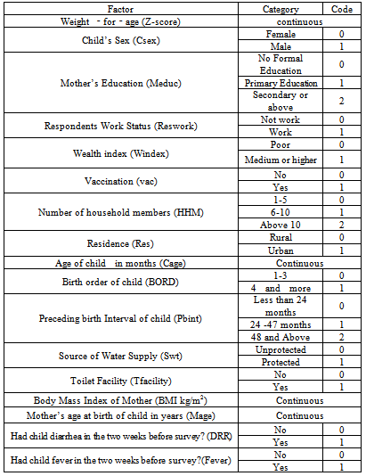
The explanatory variables which might determine nutritional status of child were socio-economic, demographic, health and environmental factors. These factors include the sex of child, age of child, preceding birth interval, birth order of child, mother’s age at child birth, place of residence, mother’s education level, mother’s work status, number of household members, household economic status, mothers body mass index, diarrhea, fever, vaccination, cough, water supply and toilet facility (Table 1).

Table 1. Explanatory Variables with their Codes

2.3. Methods of Statistical Analysis

Bayesian methods have become popular in modern statistical analysis and are being applied to a broad spectrum of scientific fields and research areas. Bayesian data analysis involves inferences from data using probability models for quantities we observe and for quantities about which we wish to learn or in other words analyzing statistical models with the incorporation of prior knowledge about the model or model parameters.

There has been much recent interest in Bayesian inference for generalized additive and related models. The increasing popularity of Bayesian methods for these and other model classes is mainly caused by the introduction of Markov chain Monte Carlo (MCMC) simulation techniques which allow realistic modeling of complex problems.

Thus, the Bayesian approach offers the viable and rigorous solution, though there is also the added benefit of providing much‐needed uncertainty and probability assessments in nonlinear and non‐Gaussian situations in a valid and rigorous way.

The statistical analysis in this research is based on Bayesian approaches which allow a flexible framework for realistically complex models. These approaches allow us to analyze usual linear effects of categorical covariates and nonlinear effects of continuous covariates within a unified semi‐parametric Bayesian framework for modeling and inference. In this work, firstly, we analyze the effects of the different types of covariates on the response variable “nutritional status” by using weight‐for‐age z‐score as continuous response variable with the assumption that each of the covariates has a linear effect on the response variable. In this case, a Bayesian Additive regression model was employed. In the first case, it assumes each covariate has a linear effect; the approach we follow in this step is Bayesian linear regression parametric approach. Secondly, since some studies suggest that body mass index and age of child as having nonlinear effect, which modify the first case, the Bayesian additive Gaussian regression parametric approach, to accommodate some transformation of these two covariates. Thirdly, to analyze the nutritional status of children we employ the same Bayesian approach, but in this case, since the three continuous covariates BMI (body mass index of the mother), Cage (age of the child), and Mage (Mother age at birth) are assumed to have a possibly nonlinear effect on the z‐score and, therefore these are modeled non-parametrically (as cubic P‐splines with second order random walk prior). Finally, it has been done by employing the Deviance Information Criteria to compare the three models.

In this study, the study proposed generalized additive models can simultaneously incorporate the usual linear effects as well as nonlinear effects of continuous covariates within a semi-parametric Bayesian approach. The inference we make is fully Bayesian and uses recent Markov Chain Monte Carlo (MCMC) simulation techniques for drawing random samples from the posterior.

2.3.1. Bayesian Structured Additive Regression Models

2.3.1.1. Generalized Additive Regression Models

Generalized Additive Models are methods and techniques developed and popularized ([14]. The study examines the generalized additive model as an alternative to the common linear model in the context of analyzing childhood nutritional status in Ethiopia. Most applications are still based on generalized linear models, assuming that covariate effects can be modeled by a parametric linear predictor. In this study, however, the data contain detailed information on continuous covariates like body mass index of the mother, mother age at child birth and child age. Their effects are often highly nonlinear, and are difficult to assess with conventional parametric models.

The generalized additive model generalizes the linear model by modeling the expected value of Y as

(1)

where, are smooth functions. These functions are not given a parametric form but instead are estimated by nonparametric methods.

While Gaussian models can be used in many statistical applications, there are types of problems for which they are not appropriate. For example, the normal distribution may not be adequate for modeling discrete responses such as counts, or bounded responses such as proportions. Thus, generalized additive models can be applied to a much wider range of data analysis problems. Generalized additive models consist of a random component, an additive component, and a link function relating these two components. Generalized additive models[14] assume that, the response Y, the random component, has density in the exponential family.

That is, conditional on covariates x_i, the responses y_i are independent and the distribution of y_i belongs to a simple exponential family, which is expressed as:

(2)

where:

is the natural parameter of the exponential family,

is a scale or dispersion parameter common to all observations, and b (.) and c (.) are functions depending on the specific exponential family.

Moreover, the conditional expectation and with link function g (.) we have

(3)

where:

X_i is the design matrix

g is the link function

The normal, binomial, and Poisson distributions are all in this family, along with many others.

The quantity in the Generalized Additive models can be expressed as

(4)

where, are smooth functions that define the additive component. Finally, the relationship between the mean μ of the response variable and is defined by a link function.

A generalized additive regression model is a special case of the generalized linear models, but they serve different analytic purposes. Generalized linear models emphasize estimation and inference for the parameters of the model, while generalized additive models focus on exploring data non-parametrically.

2.3.2. Bayesian Semi-Parametric Regression Models

The assumption of a parametric linear predictor for assessing the influence of covariate effects on responses seems to be rigid and restrictive in practical application situation and also in many real statistically complex situation since their forms cannot be predetermined a priori. In this application to childhood under-nutrition and in many other regression situations, we are facing the problem for the continuous covariates in the data set; the assumption of a strictly linear effect on the response Y may not be appropriate as suggested in[15, 16, 17].

Traditionally, the effect of the covariates on the response is modelled by a linear predictor as:

(5)

Where:

is a vector of continuous covariates,

is a vector of regression coefficients for the continuous covariates.

is a vector of categorical covariates.

is a vector of regression coefficients for the categorical covariates.

In the Bayesian parametric regression model, the parameter vectors β and γ one routinely assume diffuse priors and A possible alternative would be to work with a multivariate Gaussian distribution γ~ N (γ₀, Σ_γ0) and β ~ N (β₀, Σ _β0). However, since in most cases a non‐informative prior is desired, it is sufficient to work with diffuse priors.

In this study, the continuous covariates child’s age (Cage), the mother’s age at birth (Mage), and the mother’s Body Mass Index (BMI kg/m²) are assumed to have non-linear effects on child nutritional status. Hence, it is necessary to seek for a more flexible approach for estimating the continuous covariates by relaxing the parametric linear assumptions, by considering their true functional forms. This can be done using an approach referred to as non-parametric regression model. Non-parametric regression analysis is regression without an assumption of linearity. The scope of non-parametric regression is very broad, ranging from "smoothing" the relationship between two variables in a scatter plot to multiple-regression analysis and generalized regression models (for example, logistic non-parametric regression for a binary response variable).

To specify a non-parametric regression model, an appropriate function that contains the unknown regression function needs to be chosen. This choice is usually motivated by smoothness properties, which the regression function can be assumed to possess.

The semi-parametric regression model is obtained by extending model (5) as follows:

(6)

Where, are smooth functions of the continuous covariates.

2.3.3. Prior Distributions

Existing evidence about the parameters of interest may be available from earlier studies or from experts’ opinions and can be formalized into what is called prior distribution of the parameter of interest. A prior distribution can be non-informative, informative, or very informative. Non informative prior distributions are used in cases in which no extra-sample information is available on the value of the parameters of interest[18, 19]. In statistical terms, this lack of knowledge is represented with a distribution that attributes, approximately, the same probability to each possible parameter value.

In model (6), the parameters of interest and parameters as well as the variance parameter (τ²) are considered as random variables and have to be supplemented with appropriate prior assumptions. In the absence of any prior knowledge we assume independent diffuse priors for the parameters of fixed effects. Another common choice is highly dispersed Gaussian priors.

Several alternatives are available as smoothness priors for the unknown functions. Among the others, random walk priors[20], Bayesian Penalized-Splines[21], Bayesian smoothing splines (Hastie and Tibshirani, 2000)[22] are the most commonly used. In this study, the Bayesian smoothing spline was used by taking cubic P‐spline with second order random walk priors[23, 16].

Suppose that is the vector of corresponding function evaluations at observed values of X.

Then, the prior for f is

(8)

Where, K is a penalty matrix that penalizes too abrupt jumps between neighboring parameters. In most cases, K will be rank deficient; therefore the prior for f would be improper. This implies that follows a partially improper Gaussian prior where is a generalized inverse of a band‐diagonal precision or penalty matrix K. it is possible to express the vector of function evaluations of a nonlinear effect as the matrix product of a design matrix X_j and a vector of regression coefficients β_j,

Brezger and Lang (2006)[24] also suggest a general structure of the priors for β_j as:

(9)

where K_j is a penalty matrix that shrinks parameters towards zero or penalizes too abrupt jumps between neighboring parameters. In most cases, K_j will be rank deficient and, therefore, the prior for β_j is partially improper. The penalty matrix is of the form K = D’D, where D is a first or second order difference matrix. For example, for a p-spline with a first order random walk the penalty matrix is given by:

For full Bayesian inference, the unknown variance parameters τ² are also considered as random and estimated simultaneously with the unknown regression parameters. Therefore, hyperpriors are assigned to the variances τ² in a further stage of the hierarchy by highly dispersed (but proper) inverse Gamma priors.

(10)

A common choices for the hyperparamters are small values, for example are a=1 and b=0.005 (or b=0.0005). Alternatively, one may take a=b=0.001[21].

Priors for Fixed Effects

In the absence of any prior knowledge for the parameter vector γ of fixed effects the study considered a diffuse prior Another choice would be to work with a multivariate Gaussian distribution In this study, diffuse priors was used for the fixed effects parameter γ.

Bayesian P-spline

Any smoother depends heavily on the choice of smoothing parameters for p-spline in a mixed (fixed and continuous) framework. A closely related approach for continuous covariates is based on the P‐splines approach introduced by[25].This approach assumes that an unknown smooth function f_j of a covariate X_j can be approximated by a polynomial spline of degree l defined on a set of equally spaced knots within the domain of X_j. The domain from x_min to x_max can be divided into n’ equal intervals by d’+1 knots, Each interval will be covered by l+1 P-splines of degree l, The total number of knots for construction of the P-spline will be d’+2l+1. The number of P-splines in the regression is d’+1. It is well known that such a spline can be written in terms of a linear combination of M_j = d + l P-spline basis functions B_m, i.e.,

(11)

Here, corresponds to the vector of unknown regression coefficients. The n*m_j design matrix consists of the basic functions evaluated at the observations The crucial choice is the number of knots: for a small number of knots, the resulting spline may not be flexible enough to capture the variability of the data; for a large number of knots, estimated curves tend to over fit the data and, as a result, too rough functions are obtained. As a remedy,[25] suggest a moderately large number of equally spaced knots (usually between 20 and 40) to ensure enough flexibility, and to define a roughness penalty based on first or second order differences of adjacent P-Spline coefficients to guarantee sufficient smoothness of the fitted curves. In our analysis, we will typically choose P‐splines of degree 3 and 20 intervals, and second order random walk priors on the P‐splines regression coefficients. Hence, it is used to flexibly capture the variability of the data.

First and second order random walk priors

Let us consider the case of a continuous covariate X with equally spaced observations. Suppose that defines the ordered sequence of distinct covariate values. Here n denotes the number of different observations for x in the data set. A common approach in dynamic or state space models is to estimate one parameterfor each distinct Define and let denote the vector of function evaluations. Then a first order random walk prior for f is defined by:

(12)

The second order random walk prior for f is defined by:

(13)

With Gaussian errors u (t) ~ N (0, τ ²) and diffuse priors f (1) α const, or f (1) and f (2) α const, for initial values, respectively. A first order random walk penalizes abrupt jumps f(t) - f(t - 1) between successive states and a second order random walk penalizes deviations from the linear trend 2f(t - 1) - f(t - 2). Random walk priors may be equivalently defined in a more symmetric form by specifying the conditional distributions of function evaluations f(t) given its left and right neighbors, e.g. f(t - 1) and f(t + 1) in the case of a first order random walk. Thus, random walk priors may be interpreted in terms of locally polynomial fits. A first order random walk corresponds to a locally linear and a second order random walk to a locally quadratic fit to the nearest neighbors. Of course, higher order auto regressions are possible but practical experience shows that the differences in results are negligible[26]. The amount of smoothness is controlled by the additional variance parameter τ ², which corresponds to the smoothing parameter in a frequentist approach. The larger (smaller) the variances, the rougher (smoother) are the estimated functions. In addition, the variance τ ² controls the degree of smoothness f.

(14)

Additionally, random walk priors may be equivalently defined in a more symmetric form by specifying the conditional distributions of function f(t) given its left and right neighbors. That means, we can write the prior in (the first and second order random walk) in general form as

(15)

Here the design matrix K is the penalty matrix that penalizes too abrupt jumps between neighboring parameters. More often, K is not full rank and this implies that follows a partially improper Gaussian prior

Where, is a generalized inverse of the penalty matrix K.

For the case of non-equally spaced observations random walk priors must be modified to account for non-equal distances t = x (t)-x (t-1) between observations. Random walks of first order are now specified by f(t) = f(t - 1) + u(t); u(t)~ N(0; t τ ²); i. e. by adjusting error variances from τ ²to Random walks of second order are defined by

(16)

u(t) _~ N (0,w_t τ ²), where w_t is an appropriate weight. Several possibilities are conceivable for the weights; see[21]. However, in this analysis, we use a second order random walk prior for metrical covariates. Note that random walks are the special case of P-splines of degree zero.

2.3.4. Posterior Probability Distribution

Bayesian inference is based on the entire posterior distribution derived by multiplying the prior distribution of all parameters and the full likelihood function. For this case, let be the vector of all unknown parameters, then the posterior distribution is given by:

(17)

In many practical situations (as is the case here) the posterior distribution is numerically intractable. To overcome this problem, Markov Chain Monte Carlo (MCMC) simulation technique is used to draw samples from the posterior. From these samples, quantities such as (posterior) mean, (posterior) standard deviation, and quantiles (which in turn, gives the associated credible interval) can be estimated. Bayesian inference via MCMC is based on updating full conditionals of single parameters or blocks of parameters, given the rest and the data. For Gaussian models, Gibbs sampling with so‐called multi move steps can be applied. For non‐Gaussian responses, Gibbs sampling is no longer feasible and Metropolis Hastings algorithms are needed. More detail can be found in[27] or[21]. For the Gaussian response variable, the full conditionals for fixed effects and non-linear effects are multivariate Gaussian. For the variance parameters, all full conditionals are inverse Gamma distribution. Straight forward calculations show that precision matrices for nonlinear effects are band matrices. In fully Bayesian inference, the unknown variance parameters τ² are considered as random and estimated simultaneously with the unknown regression parameters. Therefore, hyperpriors are assigned to the variances τ² in a further stage of the hierarchy by highly dispersed inverse Gamma priors p (τ²) ~ IG (a, b).

3. Results and Discusions

3.1. Descriptive Analysis

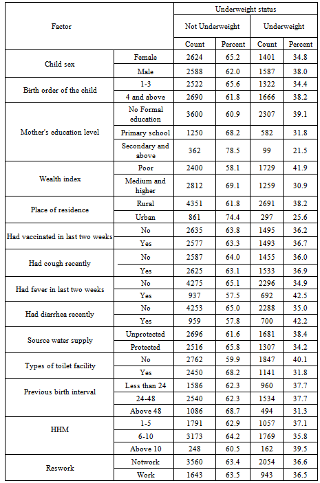
The main purpose of this study was to determine statistically the correlates of child malnutrition in Ethiopia. The data were obtained from 2011 DHS[28]. In this study a total of 8200 children under age five were considered for the analysis. Among these, 2988 (36.4%) were found to be underweight, with weight-for-age Z-score less than -2.0. This shows that underweight prevalence is high in the country. The result displayed on Table 2 shows the percentages and counts of underweight status of children with respect to the categorical explanatory variables.

As one can see from Table 2, among the 8200 cases examined in this study 38.0 % of male children were underweight and 34.8 % of female children were underweight.

In this study, birth order is recorded into two categories: first to third birth and above. As one can see from the descriptive output in most of the household the number of children ever born is greater than three. In addition to this one can easily see from Table 2 as the birth order number increase it seems that children’s nutritional status decrease.

As can be seen from Table 2, the highest prevalence of child malnutrition was observed among children whose preceding birth interval was less than 24 months (37.7%) unlike to the lowest prevalence of child malnutrition which was recorded from children whose preceding birth interval is 48 and above (31.3 %).

The proportion of underweight children, as can be seen in Table 2, differs by type of place of residence: urban and rural. Accordingly, higher numbers of underweight children (38.2%)) reside in rural areas, and relatively small numbers of underweight children (25.6%) reside in urban centers.

In this study, mother’s educational level is recorded into three categories: no formal education, primary education and secondary education and above. From Table 2, nutritional status of a child varies by educational level of mother. The highest prevalence of malnutrition was observed from children whose mothers had no formal education (39.1%) as opposed to the lowest prevalence of child malnutrition which was recorded from children whose mothers have secondary and above educational level (21.5%). It seems that a mother with higher educational level had a child with better nutritional status.

Table 2 also shows that the nutritional status of children varies by the households’ economic status. The highest probability of underweight was observed among children from poor households (41.9 %) and the lowest was noticed for children cared by non-poor household.

Households with more than 10 or more children had the highest percentage of underweight children (39.5 %) unlike to households with less than five children (37.1%).

The evidence given in Table 2 shows that the percentage nutritional statuses of children who had diarrhea recently seem to be high probability of underweight than those children which had no diarrhea recently. Likewise, one can observe that the percentages nutritional status of children who had fever recently seemed high probability of underweight than those children who have no fever recent (42.2%, 42.5 %, respectively).

The evidence given in Table 2 shows that the percentages nutritional status of children in households who had unprotected water seemed to be more severe of underweight than those children in households which used water from protected source.

3.1.1. Continuous Covariates

In this study, it seems reasonable to assume that the Z-score is (at least approximately) Gaussian distributed and, thus, model (6) could in principle be applied. Figure 1 shows a histogram estimate of the distribution of the Z‐scores of weight-for-age variable. The plots suggest that the Z-score can be reasonably approximated by a Gaussian distribution. The plot of weight‐for‐age Z-scores versus child age is given in Appendix, Figure 2. The exact shape of the influences is unknown and, hence, no simple model can be established to link the nutritional status scores to the age of the child. This effect would be explored by a nonparametric method. The plot of weight-for-age scores versus mother’s age at child birth is given in Figure 3. The plot of weight-for-age Z-score versus BMI is given in Figure 4. There is no definite pattern of relationship that can be observed from the scatter plot of body mass index (BMI) versus mean weight‐for‐age (z-score) presented in Figure 4 and this relationship can be explored by a nonparametric method.

Table 2. Distribution of Socioeconomic, Demographic, Health and Environmental related Characteristics vs Underweight (EDHS 2011)

3.2. Results of Bayesian Semi-parametric Analysis

The whole analysis has been implemented using software BayesX (Belitz Andreas Brezger, 2009)[23].

The fitted model was:

Z-score=+f₁(MBI)+f₂(Mage)+f₃(Cage)+Csexγ₁+Resγ₂+BORDγ₃+pint1γ₄+Pbint2γ₅ +HHM1γ₆+HHM2γ₇+Medu1γ₈₊Medu2γ₉+tfacilitγ₁₀+Vacγ₁₁+Coughγ₁₂+Drrhγ₁₃+feverγ₁₄+windexγ₁₅

3.2.1. Linear Fixed Effects

Table 3 gives results for the fixed effects (categorical covariates) on the nutritional status of children under age five in Ethiopia. The output gives posterior means, posterior median along with their standard deviations and 90% credible intervals. Since the 90% confidence interval do not include zero, Sex of child, birth order of child, birth interval, place of residence, cough, respondent’s current work status, mothers education level, toilet facility, household members, household economic status, diarrhea status of child and fever status of child were found statistically significant at 5% significance level. But, source of drinking water and vaccination were found statistically insignificant.

From Table 3, one can observe that having an educated mother (at least primary education) contributes to better nourishment for children under five age which has also been found in other studies[16,15]. In this study, the relative chance to be underweight for the children was found to decrease with the increase of mother’s educational level. The children of illiterate mothers and those with incomplete primary education were more likely to be malnourished as compared to mothers with secondary education and higher. The findings support the statement that educated mothers were more conscious about their children’s health[14]. Literate mothers can easily introduce new feeding practices scientifically, which helps to improve the nutritional status of children. And also the analysis shows that female children are better nourished than male children.

On the other hand, one can observe that underweight is higher for children of higher birth order (other than first born), larger household’s members, and for child residents in the rural areas. Also we observe that larger household is not conducive for better nourishment of children. However, one may interpret that while larger households provide more care to children (mostly by elder members of the household in a joint or extended family setting), there seemed to be a simultaneous competition for resources within the same larger household size. This competition for limited resources may be responsible for worsening of nutritional status for the children of a larger household size.

Household factors are strong indicators of children’s underweight status. Children in households having higher income have better nutritional status than that of lower income households. The results indicate that the risk of children being underweight decreased with the increase of household wealth index. The children of households having the lowest wealth index were more likely to be underweighted than those of household with the highest wealth index. Working status of mothers which might increase economic status of household had significant effect on child nutritional status.

The prior birth interval matters for the nutritional status of the child. The analysis showed that children born after a long birth interval were better off than other children. This statement is in agreement with[26] which found that, children with a birth interval of 2 or more years were less likely to be underweight. This may be due to the fact that the parents can take better care of fewer numbers of children and could provide adequate breast milk due to recovery of nutritional status between births. The results also indicate that source of water had no significant effect on child stunting status.

Table 3. Posterior Results of the Categorical Covariates Varname pmean pstd pqu10 Pmed pqu90 Const -0.42* 0.7 -1.1 -0.54 -0.34 Csex -0.07* 0.02 -0.1 -0.07 -0.034 BORD -0.09* 0.03 -0.13 -0.09 -0.04 Res 0.17* 0.046 0.12 0.17 0.2 Meduc0(ref) - - - - Meduc1 0.17* 0.03 0.13 0.17 0.2 Meduc2 0.45* 0.06 0.37 0.45 0.5 Swt -0.029 0.027 -0.06 -0.028 0.006 Tfacility 0.08* 0.02 0.046 0.08 0.14 HHM0(ref) - - - - - HHM1 0.03* 0.027 0.034 0.0004 0.034 HHM2 0.04* 0.06 0.16 0.04 0.038 Wealth index 0.13* 0.03 0.09 0.135 0.17 Reswork 0.002* 0.026 0.03 0.001 0.03 DRR -0.02* 0.22 -0.02 -0.31 -0.45 Fever -0.27* 0.22 -0.56 -0.27 -0.027 Pbint1(ref) - - - - - Pbint1 0.024* 0.031 0.015 0.023 0.06 Pbint2 0.13* 0.13 0.056 0.08 0.14 Cough -0.06* 0.12 -0.32 -0.22 -0.06 Vaccination 0.044 0.12 -0.19 -0.12 0.045

3.2.2. Non-linear Effects under Generalized Additive Linear Regression Models

Nonlinear effects represented by smoothed functions, are commonly interpreted graphically. Figure 5 shows the smooth function of the children age versus weight‐for‐age z-score. The posterior means together with 80% and 95% point wise credible intervals are shown. One can observe that the influence of a child’s age on its nutritional status is considerably high in the age range between the ages of 0-27 months with decreasing trend; and then stabilizes.

As suggested by the nutritional literature, one can able to distinguish the continuous worsening of the nutritional status up until about 27 months of age. This deterioration set in right after birth and continues, more or less linearly, until 27 months. After 27 months the effect of age on underweight stabilizes at a low level. Through reduced growth and the waning impact of infections, children were apparently able to reach a low‐level equilibrium that allows their nutritional status to stabilize[21, 14, 23, 21].

Figure 6 displays nonlinear effects of mother’s age at birth in years. It shows the posterior means together with 80 % and 95% point-wise credible intervals. It is evident from the analysis that increasing age of mother at birth reduces underweight status of children. That is younger mothers tend to have more underweighted children than older mothers. Mother age at birth shows significant effect on underweight status of children under age of five years old. The effect of mother’s age on her child’s underweight status (other constant) negatively increase as her age increase up to 25 years and then after the effect of mothers age on her child’s underweight status positively increase.

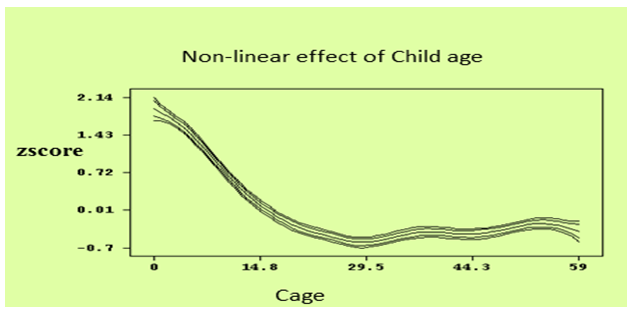Figure 5. Non-linear Effects of Child’s Age in months on Nutritional Status of a Child

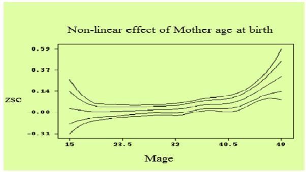Figure 6. Non-linear Effects of Mother’s Age in years on Nutritional Status of a Child

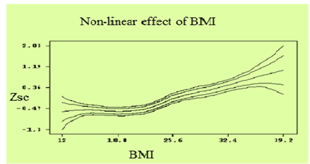Figure 7. Non-linear Effects of Mother’s Body Mass Index (kg/m2) on Nutritional Status of a Child

Figure 7 shows the flexible modelling of the effect of the BMI kg/m² of the mother versus underweight. The posterior means together with 80 % and 95% point wise credible intervals are displayed. Bearing in mind at the mother’s BMI kg/m² and its impact on the level of nutritional status, it was found that the influence had a regular pattern. The underweight status of a child improves as mothers BMI increases. In general, the figure shows that BMI kg/m² had a significant effect on child nutritional status.

3.3. Discussion

This study was intended to identify the determinants of the underweight status of children under five years old in Ethiopia based on EDHS 2011 data. The nutritional status was measured by the weight-for-age. Accordingly, Bayesian semi-parametric regression analysis on underweight was employed to identify flexibly the effect of covariates on nutritional status of the children. In this study, underweight was analyzed based on the modified anthropometric measurement indicators of the nutritional status of children calculated using new growth standards published by the World Health Organization in 2006. The results obtained are discussed as follows. The total number of children covered in the present study was 8200, among which 36.4 % were underweight. The Bayesian semi-parametric analysis revealed that the covariates: sex of child, birth order of child, place of residence, cough, previous birth interval, mothers education level, toilet facility, household members, household economic status, diarrhea and fever were found statistically significant. But, source of drinking water and vaccination were found statistically insignificant (though not expected).

Preceding birth interval is an important demographic variable that affects nutritional status of children. As the preceding birth interval increases, the nutritional status of a child increases. This finding is confirmed by most of previous studies[19, 21, 13]. The significant and higher risk of underweight among children of lower preceding birth interval could be due to uninterrupted pregnancy and breastfeeding, since this drains women’s nutritional resources. Close‐spacing may also have a health effect on the previous child who may be prematurely weaned if the mother becomes pregnant too early again.

The fact that mother education level was significant is in agreement with different reports under taken on the same problem. According[28], with an increase in mothers’ educational level, incidence of malnutrition among young children decreases. And this factor is then directly associated to the women’s own nutritional status and quality of care they receive[39]. The educated mothers are more conscious about their children’s health. Literate mothers can easily introduce new feeding practices scientifically, which help to improve their children nutritional status[26].

Household economic status is also an important socio - economic variable that affects nutritional status of children in Ethiopia. Children in poor households were found to be at a higher risk of malnutrition problem than children from rich households. This finding is consistent with other studies[19, 11]. The study indicated that better off households had better access to food and higher cash incomes than poor households, allowing them a quality diet, better access to medical care and more money to spend on essential non-food items such as schooling, clothing and hygiene products.

As the study has revealed that, household size is an important variable that affects nutritional status of children. The prevalence of underweight increased with increasing household size. Households with more than 10 and above child had a higher percentage of underweight children (39.5%) compared with households with less than five children (37.1 %). Large household size is not conducive for better nourishment of children. However, we may interpret that while larger households provide more care to children (mostly by elder members of the household in a joint or extended family setting), there seemed to be a simultaneous competition for resources within the same larger household size. This competition for limited resources may be responsible for worsening of nutritional status for the children of a larger household size. This result is in agreement with a study under taken by[31] which stated that children living in a household with only one child have a lower risk of nutrition than children who live in households with more than one child. The total number of children within a household influences the resources available to each child, in terms of financial, time and attention. In a crowded household, exposure of an individual child to infection is also increased[32].

As shown in the analysis, urban children were less likely to be malnourished than their rural counterparts because the quality of health environment and sanitation is better in urban areas, whereas, the living condition in rural areas were associated with poor health condition, and lack of personal hygiene, which were the risk factors in determining malnutrition. This is consistent with some studies, where mothers’ place of residence has a statistical significant effect on children nutritional status[27, 11].

The findings of this study also showed that children who had diarrhea two weeks before date of survey are vulnerable to malnutrition problem than those who had not. This finding is consistent with other studies[13, 33, 34]. This may be due to the fact that diarrhea accelerates the onset of malnutrition by reducing food intake and increasing catabolic reactions in the organism. Diarrhea also affects both dietary intake and utilization, which may have a negative effect in child nutritional status. The type of toilet used by a household is an indicator of household wealth and a determinant of environmental sanitation. This means that poor households were less likely to have sanitary toilet facilities. In consequence, these results increased risk of childhood diseases, which contribute to malnutrition.

It is evident that increasing age of mother’s at birth reduces underweight and shown that children whose mothers are older age group were better in their underweight status as compare to children whose mothers are in the younger age group. The mother’s age at birth of the index child was found to be a statistically significant predictor of children’s underweight status in a number of previous studies, where it was found that children born to mothers between the ages of 20 and 29 years were more likely to have children that suffered from negative nutritional outcomes than those children born to older mothers[35]. Children whose mothers are older than 30 years of age are better in their stunting status as compare to children whose mothers are in the younger age group[14].

In the study, the effect of the age of the child is obviously nonlinear and decreasing between birth and an age of about 20 months and then stabilizes. That means the underweight of children increases until 24 months. This continuous worsening of the nutritional status may be caused by the fact that most of the children obtain liquids other than breast milk already shortly after birth. After 24 months a relatively stable, low level is reached. However, it reaches its minimum level between ages 24-30 months, then rises again and stabilizes thereafter at a middle level with a bump till 5 years. Previous studies also confirm this[27, 13, 14].

Mother’s body mass index is defined as her weight in kilo‐grams divided by her square of her height in meters. Mothers with low BMI value are themselves malnourished and are therefore likely to have undernourished children. The same finding is also found in a number of studies. Mothers with low BMI on average giving birth to babies of low birth weight[14].

4. Conclusions

The main objective of this study was to identify the most important predictors of under five years old children underweight status in Ethiopia using Bayesian Semiparametric regression model. The study revealed that socio-economic, demographic and health and environmental variables have significant effect on the underweight status of children in Ethiopia. Using Bayesian Semiparametric regression model, the predictors, sex of child, birth order of child, preceding birth interval, place of residence, cough, mother’s education level, toilet facility, household members, household economic status, diarrhea and fever are the most important determinants of child underweight status in the country.

The study showed that children from uneducated mother, lower preceding birth interval (less than 24 months), higher birth order, economically poor household, large household size are more vulnerable to underweight problem in Ethiopia. The findings of this study also showed that children who had diarrhea and fever for two weeks before the date of survey are significantly vulnerable to underweight problem than those who had not. Male children are more vulnerable to underweight problem than female children.

The study analyzed how the continuous covariates: child's age, mother's age at birth and mother's BMI affect underweight status of the child. The underweight status of a child improves as mother’s body mass index increases. And children are at high risk of underweight problem during the first 0‐24 months of their life and then stabilize moderately with bump. The study also revealed that children whose mothers are in the older age group are better in their nutritional status as compare to children whose mothers are in the younger age group.

Appendixes

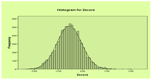Figure 1. Histogram for Zscore

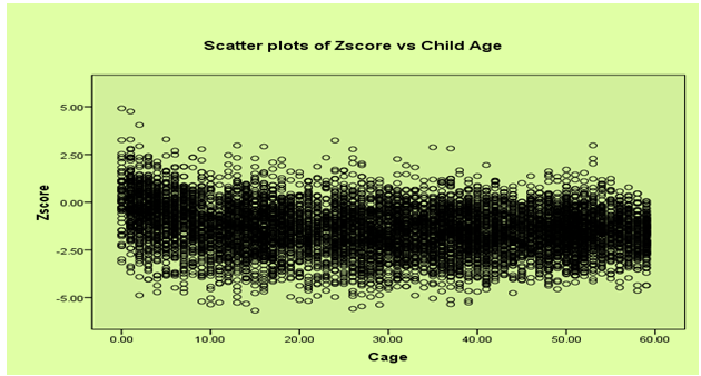Figure 2. Scatter plots of Zscore vs Child Age in months

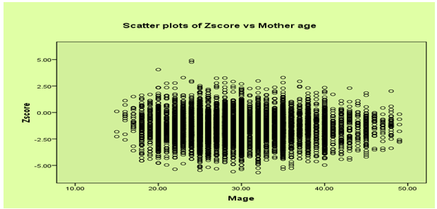Figure 3. Scatter plots of Zscore vs mother age at child birth in years

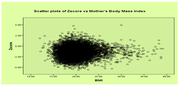Figure 4. Scatter plots of Zscore vs Mother’s Body Mass Index (kg/m2)