E. P Sreedevi, P. G. Sankaran
Department of Statistics, Cochin University of Science and Technology, Cochin, 682022, India
Correspondence to: E. P Sreedevi, Department of Statistics, Cochin University of Science and Technology, Cochin, 682022, India.
| Email: |  |
Copyright © 2012 Scientific & Academic Publishing. All Rights Reserved.
Abstract
Modeling and analysis of lifetime data using neural network models is a topic of recent interest in survival studies. In the present study, we use multilayer perceptron neural network models for the analysis of competing risks data. Multilayer perceptron neural network with a modification is used for the estimation of survivor function in presence of covariates. The estimates are compared to the smoothed estimates proposed by Wells[1], by extending the procedure into the competing risks set up. Neural network models are also used for classification of failure types in competing risks data. We illustrate the methods using real data sets.
Keywords:
Classification, Competing Risks Models, Cox Proportional Hazards Model, Multi-layer Perceptron, Neural Networks
Cite this paper: E. P Sreedevi, P. G. Sankaran, Analysis of Competing Risks Data Using Neural Network Models, International Journal of Statistics and Applications, Vol. 3 No. 4, 2013, pp. 123-131. doi: 10.5923/j.statistics.20130304.05.
1. Introduction
In life testing experiments, the death (failure) of an individual either a living organism or an inanimate object, may be classified into one of  mutually exclusive classes, usually cause of failure. For example, cause of death of an individual may be classified as cancer, heart disease or other. Competing risks models are useful for the analysis of such data in which an object is exposed to two or more causes of failure. The competing risks models also arise in public health, demography, actuarial science, industrial reliability applications and experiments in medical therapeutics.In literature, various techniques are available for the analysis of competing risks data. Non-parametric methods are more popular in survival studies due to the fact that the lifetime data may not always meet parametric model assumptions. Gasbarra and Karia[2], Crowder[3], Kwam and Singh[4] and Lawless[5] provide comprehensive reviews on this topic.Neural networks (NN) are one of the most widely used non parametric methods in the analysis of lifetime data. Multi-layer perceptron (MLP) networks are the most commonly used neural network models in survival studies. The basic element of a neural network model is a single unit perceptron. A single perceptron, can be treated as a regression model, represented by
  where
where  is the expected response
  is the input response ,
 s are corresponding weights and
  is the added bias. For more details, see Cheng and Titterington[6].MLP neural network models are employed in survival studies to improve estimates of survivor function (see Bakker and Heskes[7] and Bakker et al.[8]). Recently Biganzoli et al.[9] used partial logistic artificial neural networks to model competing risks data in the discrete set up. Ambrogi et al.[10] discussed the use of neural network models with genetic algorithms to solve various problems in classical survival analysis. One can refer to MacKay[11], Ravdin and Clark[12], De Laurentiis and Ravdin[13], Faraggi and Simon[14], Bishop[15], Neal[16], Ripley[17], Ripley and Ripley[18], Neal[19], Biganzoli et al.[20,21], Eleuteri et al.[22,23], and Ahmed[24] for various applications of neural networks in survival analysis. The main advantage of neural network models over traditional statistical models is the flexibility they offer. The heuristic and algorithmic approach helps to solve complexities beyond the reach of empirical statistical methods. In the present study, we discuss the analysis of competing risks data using MLP neural network models. The text is organized as follows. In Section 2, we describe the basic concepts of competing risks models. Section 3, introduces a neural network model for the analysis of competing risks data. The estimates of cumulative cause specific hazard rate functions and cause specific subdistribution functions are given. The analysis of competing risks data in the presence of covariates is discussed in Section 4. We develop a neural network model for the estimation of survivor function and illustrate the procedure with real data set given in Andersen et al.[25]. Cause specific subdistribution functions are also estimated using the neural network model proposed in Section 3. Wells[1] proposed a smoothing technique for baseline hazard rate function estimation. We extend this idea into competing risks set up and the neural network estimates are compared with the corresponding smoothed estimates. In Section 5, we employ neural network models for classification of failure times according to the cause of failure. A sensitivity-specificity analysis is carried out to assess the accuracy of the classification. Finally, Section 6 provides a brief conclusion of the study.
2. Competing Risks Models
Two frame works are often used to deal with standard competing risks settings in which a life time variable  and a cause of failure
  can be observed for an individual:
 Cause specific hazard rate funcion
 formulations, where
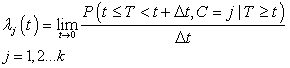 | (2.1) |
and Cause specific subdistribution function
  formulations, where
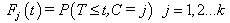 | (2.2) |
 is the instantaneous rate of failure of type
  at time
  given the individual has survived time and in the presence of all other failure types. Comparison of cause-specific subdistribution functions is useful in selecting appropriate treatment for a patient Kalbfleisch and Prentice[27]. Either set of these functions fully specify the joint distribution of
  and
and  , but they lead to different types of regression models when covariates are present. For more properties and applications of (2.1) and (2.2), one can refer Kalbfleisch and Prentice[27].Nelson-Aalen (NA) non-parametric estimator for the cumulative cause specific hazard rate function
  is given by
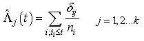 | (2.3) |
where  is the number of patients alive and uncensored just prior to time
  and
and  is the indicator variable defines as
  with
with  as the cause of death of
  th individual for
  .In competing risks set up, we assume that the
  failure types are mutually exclusive and exhaustive so that an individual can have at most one realized lifetime. Then the overall hazard rate function
  is given by
 | (2.4) |
Thus from (2.3), the survivor function and cause specific subdistribution functions can be estimated as  | (2.5) |
and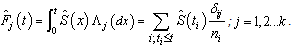 | (2.6) |
In survival studies, covariates or explanatory variables are employed to represent the heterogeneity in a population. The main objective in such situations is to understand and exploit the relationship between the lifetime and explanatory variables. The proportional hazards (PH) model proposed by Cox[28] is the well-known semi parametric regression model that is widely employed in such contexts. This model is used in the competing risks situation by considering  | (2.7) |
where  is the
  vector of covariates and
  is a
is a  vector of regression coefficients,
  is the cause specific hazard rate function in presence of covariate vector
  and
and  is the baseline cause specific hazard rate function common to all patients. The estimation of
  can be done by maximizing partial likelihood function(see Lawless[5]). The cumulative cause specific hazard rate function
  is estimated by
 | (2.8) |
which is an extension of the NA estimator of cumulative hazard rate function, where  , if
, if  th individual is alive and uncensored at time
  and 0, otherwise.Using counting process approach, we can represent (2.8) as
  | (2.9) |
where,  with
with  counts the observed events on
  th individual at time
  .By extending the idea given in Wells[1] into competing risks set up, the estimate of the baseline cause specific hazard rate function is given by
  | (2.10) |
where,  is a density function on
  , symmetric about zero, with unit integral and
  is a sequence of positive numbers tending to zero. In the present study, we consider
  and
and  is chosen in such a way that the mean square error of the estimates is minimum.Consequently,
  is estimated using (2.5) and (2.7) as
  | (2.11) |
Cause specific subdistribution functions can be estimated using (2.11) by | (2.12) |
The semi parametric model described above is distribution free in the sense that their validity and certain properties do not depend on the true form of  , provided the multiplicative form is correct. However, this multiplicative form is a strong assumption which may violate in many situations.In the following section, we discuss the estimation of cumulative cause specific hazard rate functions and cause specific subdistribution functions using neural networks models.
3. Estimation Using Neural Network Models
MLP neural network with one hidden layer, with one neuron in the hidden layer is used in this study. Since increasing the number of hidden neurons is only recommendable for handling complex situations, simplest structure of the network is used here. For the estimation of cumulative cause specific hazard rate functions, lifetime and cause of failure are given as input variables. Censored observations are accommodated in the analysis by denoting them with a cause labeled ‘0’. Hidden and output units use two functions viz. combination functions and activation functions to produce their outputs. All the computed values from previous units are fed into the given unit and combined into a single value using a combination function. The value produced by the combination function is transformed by an activation function (transfer function). Linear general combination function and exponential transfer function are used in the analysis. Linear general combination function is given as where
where  is the input of the
  th neuron,
  is the weight connecting
  th and
  th neurons,
  is the bias of the
  th neuron and
  is the
  th neuron’s output.
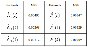
 Table 1. Estimates of MSE of
 and and
 for Hoel’s data set, for Hoel’s data set,

 |
| |
|
Activation functions are selected according to target variables. For the estimation of cumulative cause specific hazard rate functions, we use exponential activation function. Normal error function is used in our model, since it is the most appropriate error function for interval type target variables. Another possible choice of error function, Poisson error function is not considered here, since the target variables don’t follow the Poisson distributional property of equality of mean and variance. The MLP networks we trained here are of small or medium sized networks, which have only a small number of connections. So we use Quasi-Newton learning algorithm to train the networks, since the memory storage will not be a problem for such networks. Neural networks are trained by minimizing an objective function. The likelihood function is used as the objective function for optimization. The model complexity is controlled using the weight decay method, with weight decay constant 1. In a similar fashion, cause specific subdistribution functions can also be estimated, with the change in transfer function only. Logistic transfer function is used in the output layer to restrict the output between 0 and 1. Estimates of cumulative cause specific hazard rate functions and cause specific subdistribution functions are given as target variables. For illustration purpose, a competing risks data set given by Hoel[29] is considered. The data are obtained from a laboratory experiment on RFM strain male mice, which had received a radiation dose of 300 rads at ages of 5 to 6 weeks and were kept in a conventional germ-free environment. There are three causes of death viz. thymic lymphoma, reticulam cell sarcoma and other causes. All mice died by the end of experiment, so there is no censoring. The data set contains 181 time points and is divided into training and validation data sets. The training set consists of 80% of the data points which is used for preliminary model fitting and validation set contains the other 20% which is used to assess the adequacy of the model. Mean square error (MSE) of the neural network models in the last iteration for estimating cumulative cause specific hazard rate functions and cause specific sub distribution functions for the Hoel’s data set is given in Table 1. The plots of estimated values of cumulative cause specific hazard rate functions and cause specific subdistribution functions for two causes are also given in Figures 1 (a)-1 (c). In Figures 1 (a)-1(c), dark line represents the smoothed statistical estimates and dotted line represents the corresponding neural network estimates.Figures 1(a)-(c) and 2 (a)-(c) compare the smoothed estimates using non parametric methods and neural network method of cause specific sub distribution functions. Neural network model gives smoothed estimates of cause specific sub distribution functions without using any other smoothing techniques.
4. Competing Risks Situation with Covariates
In Cox proportional hazards model, the hazard rate function consists of two independent parts. The first part is,  , in which depends on patient information, say covariates
  only and the second part is the time dependent base line hazard rate
  .
.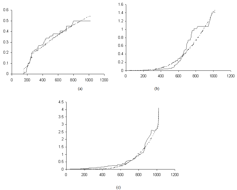 | Figure 1(a)-(c). Plots of the estimates of cumulative cause specific hazard rate functions for mice died of thymic lymphoma, reticulum cell sarcoma and other causes |
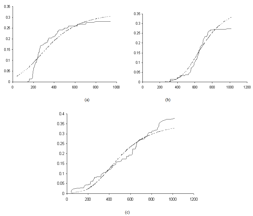 | Figure 2(a)- (c). Plots of the estimates of cause specific subdistribution functions for mice died of thymic lymphoma, reticulum cell sarcoma and other causes |
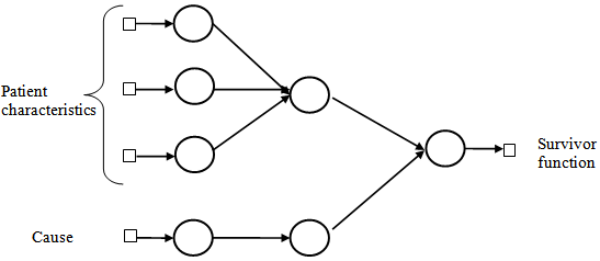 | Figure 3. Architecture of a multi-layer perceptron network used for estimation of survival probability in competing risks set up |
Cox proportional hazards model is implemented in an MLP with one hidden unit and  output units, specifying the survivor function
  at
at  discrete points of time. Patient characteristics are given as input variables. The input to hidden weights are denoted by
  and hidden to output layer weights by
  . All the units have exponential transfer functions. In the first step, the output of the hidden unit is
  , where
  represents a vector of unknown regression coefficients. In the second step, the output of th target node is
  which is the survival probability with
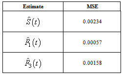
  .In competing risks situation, we add one more input node to this frame work, cause of failure and treat it as ordinal variable. In hidden layer, one more neuron is added with logistic activation function, which is connected to target nodes (see Figure 3). This network estimates the survivor function in presence of covariates.To implement this network, we consider the data set given in Andersen et al.,[25]. The data consists of survival times of 202 melanoma patients with cause of death and covariates age, sex, an indicator variable of patient’s condition, year of operation, tumor thickness and ulceration. We consider three covariates in this study namely, age, sex and tumor size of the patient for illustration. The covariate age is in years, sex (1-man, 0- woman) and survival time in days. C=1 (death from malignant melanoma); C=2 (alive on 1, Jan 1978); C=3 (death from any other causes). Neural network model proposed in Section 3 is used to estimate cause specific sub distribution functions, where patient characteristics are also given as input variables. Mean square error of the neural network models in the last iteration for estimating survivor function and cause specific subdistribution functions for the melanoma data set is given in Table 2. Figure 5 compares the smoothed estimates and neural network estimates of survivor function. Figures 6 (a)-(b) plots the smoothed non parametric estimates and neural network estimates of cause specific subdistribution functions. In Figures 5 and 6(a)-(b) dark line represents smoothed statistical estimates and dotted line represents the corresponding neural network estimates.
Table 2. Estimates of MSE of
 and and
 for melanoma data set, for melanoma data set,

 |
| |
|
From Figure 4, it follows that the absolute difference between two estimates of survivor function exceeds 0.1 only for three data points. The maximum difference obtained is 0.2578. This corresponds to the value 17.42, for the covariate tumor thickness, where as the average value of tumor thickness for patients is 2.906. Considering the other two data points, for which the absolute difference between estimates exceeds 0.1, the value of covariate variable tumor thickness exceeds 10. These observations show that, the two estimates are almost equally reliable for estimation. But, it should be noted that for those data points which deviate extremely from the average value of the input variable age, the estimates of survivor probability do not show much deviation. Thus it follows that the value of covariate, tumor thickness, has high influence on estimated values. 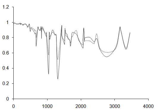 | Figure 4. Plot of survivor function ( including covariate effect) for melanoma data set |
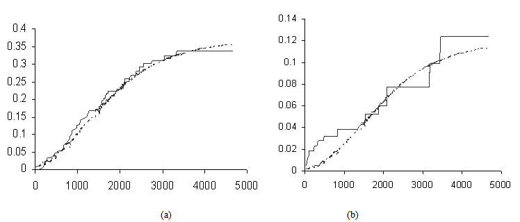 | Figure 5(a)-(b). Plots of the estimates of cause specific subdistribution functions for melanoma data |
From Figures 5(a)-(b), it follows that neural network model provide smoothed estimates cause specific subdistribution function.
5. Classification Problems
In this section, we present neural network models for two different classification problems in competing risks set up. We consider the situations in presence of covariates.
5.1. Binary Model Network
We present a neural network model to estimate the survivor probability within a pre specified time point and hence to classify the individuals into two groups at any specified time point according to whether the individual is survived or relapsed. We modify the data by splitting the time into two periods, before the pre specified time point and after the pre specified time point. This model is a standard classification neural network. This model is an extension of the binary model introduced by Ripley et al.[30] into the competing risks set up.Let  denote the pre specified time point. Assume that
  be the probability of relapse for
  th patient due to cause
  before
  and
and  be the indicator variable which equals 1 if
  th patient is relapsed due to cause
  before
  and 0 otherwise.Now the likelihood function of the observed data is given by
 where
where  and
and  with
with  and
and  .To incorporate censorship, we follow[31]. Each censored patient is included twice in the data, with indicator 1 and 0 with appropriate weights. We have used multilayer perceptron network with one hidden layer and logistic activation functions.
5.2. Softmax Neural Network
In the following, we present a softmax neural network to classify the individuals into different groups according to their causes of death. The individual’s survival time or censoring time and the explanatory variables are given as inputs. Censored individuals are considered as a separate class. Target variable is the indicator function denoting the class membership. The model is fitted with cross entropy error function and softmax activation function. With a softmax activation function, the probability of the membership for class  is given by
 where
where  is the output from the previous unit.For illustration of classification problems, we use the same mice mortality data due to Ripley et al.[30]. Living environment of the mice is selected as covariate. The accuracy of the classification is assessed in terms of sensitivity and specificity. Sensitivity is the proportion of event responses that are predicted to be events and specificity is the proportion of non-event responses that are predicted to be non-events. The time point is selected as 550 days and we run the binary model to predict the survival before 550 days for three observed causes. The sensitivity and specificity of the model is calculated using a 0-1 loss function. The results of the classification in terms of sensitivity and specificity are given in Table 3. Both models seem to yield best results regarding classification.
 | Table 3. Sensitivity and Specificity based on a 0-1 loss function for the binary model |
| | Cause | Sensitivity | Specificity | | Thymic lymphoma | 94.1 | 45.9 | | Reticulum cell sarcoma | 93.2 | 44.6 | | Other causes | 95.4 | 49.0 |
|
|
To assess the accuracy of classification using softmax neural network models, we calculate the specificity and sensitivity based on a 0-1 loss function. The results are given in Table 4.| Table 4. Sensitivity and Specificity based on a 0-1 loss function for softmax neural networks |
| | Cause | Sensitivity | Specificity | | Thymic lymphoma | 87.7 | 75.8 | | Reticulum cell sarcoma | 82.3 | 73.4 | | Other causes | 91.2 | 78.7 |
|
|
6. Conclusions
In the present work, we proposed neural network models for various estimation and classification problems in the analysis of competing risks data. Multiple time point neural network models are developed to estimate cumulative cause specific hazard rate functions, cause specific subdistribution functions and survivor functions. When covariates are present, we introduced a multilayer perceptron neural network model for the direct estimation of survivor probability. We extended the smoothing procedure proposed by Wells[1] into competing risks set up and compare the smoothed estimates with the same given by neural network models. It has been shown that neural networks give the smoothed estimates inherently without using any other smoothing techniques. Another important advantage of the neural network models is that, they are free from any assumption about the distribution of data. The flexibility that the neural network models offer for modeling the data is also an additional advantage. The heuristic and algorithmic approaches help us to solve complexities in the real life situation that are beyond the reach of empirical statistical methods. However, neural network models bear their inherent drawback of being data dependent.We, further proposed a binary model to classify individuals into two groups of survived and relapsed patients at a pre specified time point. A softmax neural network model was also employed to classify the individuals according to their cause of failure. Classification of failure times according to the cause of failure is important in testing the independence of time of failure and cause of failure. Since the dependent structure of time to failure and cause of failure is important in competing risks analysis, neural network models for this problem are of greatest importance. Works in this direction will be reported elsewhere.
References
| [1] | Wells. M. T. (1994): Non parametric kernel estimation in counting processes with explanatory variables. Biometrika. 81 795-801. |
| [2] | Gasbarra.D. and Karia. S.R.(2000): Analysis of competing risks using Bayesian smoothing, Scandinavian Journal of Statistics. 27 605-617. |
| [3] | Crowder. M. (2001): Classical Competing Risks. Chapman and Hall, London . |
| [4] | Kwam. P.H. and Singh. H. (2001): On nonparametric estimation of the survival function with competing risks. Scandinavian Journal of Statistics. 28 715-724. |
| [5] | Lawless. J .F.(2003): Statistical Models and Methods for LifeTime Data. John Wiley and Sons, New York. |
| [6] | Cheng. B. and Titterington. D. M.(1994): Neural networks: A review from a statistical perspective. Statistical Sciences. 9 2-54. |
| [7] | Bakker.B. and Heskes. T.(1999): A neural Bayesian approach to survival analysis. International Conference in Artificial Neural Networks. Conference Publication No:470. |
| [8] | Bakker.B., Heskes. T., Neijit J. and Kappen. B.(2001): Improving Cox survival analysis with a neural Bayesian approach. Statistics in Medicine. 23 2989-3012. |
| [9] | Biganzoli. E., Boracchi. P., Mariani.L. and Marubibi.E. (1998): Feed forward neural networks for the analysis of censored survival data: A partial logistic regression approach. Statistics in Medicine. 17 1169-1186. |
| [10] | Ambrogi. F., Lama. N., P. Boracchi. P. and Biganzoli. E.(2007): Selection of artificial neural network models for survival analysis with genetic algorithms. Computational Statistics and Data Analysis. 52 30-42. |
| [11] | MacKay. D. J. C.(1992): A practical Bayesian framework for back propagation networks. Neural Computation. 4 448–472. |
| [12] | Ravdin. P. M. and Clark. G.M.(1992): A practical application of neural network analysis for predicting outcome of individual breast cancer patients. Breast Cancer Research and Treatment, 22 285-293. |
| [13] | De Laurentiis. M. and Ravdin. P.M. (1994): A technique for using neural network analysis to perform survival analysis of censored data. Cancer letters. 77 127-138. |
| [14] | Faraggi. D. and Simon. R.(1995):. A neural network model for survival data. Statistics in Medicine. 14 73–82. |
| [15] | Bishop. C. M. (1996): Neural Networks for Pattern Recognition. Oxford: Clarendon Press. |
| [16] | Neal. R. M. (1996): Bayesian Learning for Neural Networks. New York, Springer. |
| [17] | Ripley. B. D., and Ripley. R.M.(1998): Neural networks as statistical methods in survival analysis. Artificial neural networks: Prospects for medicine (R. Dybowsky and V. Gant eds.). Lands Biosciences, Publishers. |
| [18] | Ripley. R.M.(1998): Neural network models for breast cancer prognosis. PhD Thesis, Department of Engineering Science, University of Oxford. |
| [19] | Neal. R. M.(2001): Survival analysis using a Bayesian neural network. Joint Statistical Meetings Report, Atlanta. |
| [20] | Biganzoli.E., Boracchi. P. and Marubini. E.(2002): A general framework for neural network models on censored survival data. Neural Networks.15 209–218. |
| [21] | Biganzoli. E., Boracchi. P., Ambrogi. F. and Marubini. E.(2006): Artificial neural networks for the joint modeling of discrete cause specific hazards. Artificial Intelligence in Medicine. 37 119-130. |
| [22] | Eleuteri.A., Tagliaferri.R., Milano.L.,De Placido.S. and De Laurentiis. M.(2003): A novel neural network based survival analysis model. Neural Networks. 16 855-864. |
| [23] | Eleuteri.A., Tagliaferri.R., Milano.L., Sansone. G., D’agostino. D., De Placido.S. and De Laurentiis M.(2003):. Survival analysis and neural networks. Proceedings of the International Joint Conference on Neural Networks. 4 2631-2636. |
| [24] | Ahmed. F. E.(2005): Artificial neural networks for diagnosis and survival prediction in colon cancer. Molecular Cancer, 4 29-41. |
| [25] | Andersen P. K., Borgan O., Gill. R. D. and Keiding. N.(1993): Statistical Model Based on Counting Process. Springer- Verlang, New York . |
| [26] | Gray. R. J.(1988): A class of k-sample tests for comparing the cumulative incidence of a competing risks. The Annals of Statistics. 16 1141-1154. |
| [27] | Kalbfleisch. J. D. and Prentice. R. L.(2002): The Statistical Analysis of Failure Time Data. John Wiley and Sons, New York. |
| [28] | Cox. D. R.(1972): Regression models and life tables. Journal of the Royal Statistical Society Series- B. 34 187-220. |
| [29] | Hoel. D. G.(1972): A representation of mortality data by competing risks. Biometrics.28 475-488. |
| [30] | Ripley, R.M., Harris, A. L. and Tarassenko, L. (2004): Nonlinear survival analysis using neural networks. Statistics in Medicine. 23 825-842. |
 Abstract
 Reference
 Full-Text PDF
 Full-text HTML