1. Introduction

Longitudinal studies are often used in public health and medical sciences. Such studies are often designed to investigate changes in a specific variable, which is measured repeatedly over time for every participant. A typical example of longitudinal studies is to measure blood pressure for patients with hypertension several times during a specific period of time. In fact longitudinal studies are powerful design since they are measuring the changes of the variable of interest over time.

Longitudinal studies are rarely complete due to patient attrition, mistimed visits, premature study termination, death, and other factors. Missing data in longitudinal studies can be a difficult problem to overcome. Although investigators may devote substantial efforts to minimize the number of missing values, some amount of missing data is inevitable in the practice. Missing data could be in the response variable, the covariates, or both. Our interest is on the missingness in the response variables.

A vast amount of work has been done in the area of missing values, see for example Fitzmuarice et al.[1] and references therein. This has led, on the one hand, to a rich taxonomy of missing data concepts, issues, and methods, and, on the other hand, to a variety of data-analytic tools. If missing data are treated inadequately, the statistical power of detecting treatment effects may be reduced, the variability might be underestimated and bias may affect the estimation of the treatment effect, the comparability of the treatment groups, and the generalizability of the results. So, it might be necessary to accommodate missing values in the modelling process to avoid either biased parameter estimates or invalid inferences.

The missing data pattern can be categorized into two patterns: intermittent missing values (i.e., missing values due to occasionally withdrawal) with observed values afterwards, intermittent missingness is also termed non-monotone missing pattern, and dropout (i.e., missing values due to earlier withdrawal), with no observed values. Dropout missing pattern is monotone pattern ([2];[3]).

Let be the response for the measurement from the subject, made at time 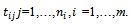The times are assumes to be common for all subjects. Let 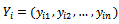be the vector contains the response of the ith subject at all times. Assume that the vector of responses can be partitioned to the observed part and the missing part, i.e. The impact of missing data and the ways to handle incomplete data depend much upon the mechanism of incompleteness. A set of definitions for missing data mechanisms has been proposed by Rubin[4], also in[5]. These aremissing completely at random (MCAR), missing at random(MAR), and missing not at random (MNAR). They introduce an indicator variable where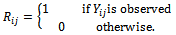

The missing data are missing completely at random (MCAR), if the random variable is independent of both in notation:

i.e., If the missingness is independent of both unobserved and observed data. If the missingness in not related to the data being missing, conditional on the observed measurements, this called missing at random (MAR). i.e., if the random variable is independent of

If the missingness also depends on the unobserved data it is considered to be missing not at random (MNAR) also called (informative). Informative missingness refers to the fact that the probability of missingness depends on the underlying individual characteristics. i.e., the random variable is conditionally dependent on given

When data are MNAR valid analysis requires explicit incorporation of the missing data mechanism, which in most situations will be unknown. That is because under informative missingness, the estimation methods ignoring missing data process can lead to severely biased estimators ([6];[7]).

Imputation techniques have become an important and influential approach in the statistical analysis of incomplete data. The imputation techniques can be classified according to the number of imputed values as single imputation (SI) and multiple imputations (MI). In single imputation techniques each missing observation is replaced by a single value. In multiple imputation techniques each missing value is imputed by a group of observations[8,9]. Standard statistical analysis is carried out on each imputed data set, producing multiple analysis results. These analysis results are then combined to produce one overall analysis.

The key advantages of MI are flexibility and simplicity. It applies to a wide range of missing data situation and is simple enough to be used by non-statisticians. Theoretically this approach is superior to other models because it often produces the most robust effects[7]. The second advantage is bias correction. When the missing data mechanism is MAR, as opposed to MCAR, the method corrects for biases in complete case analysis and other ad hoc analyses[6];[10]. Moreover, auxiliary variables that are not part of the analysis procedure can be incorporated into the imputation procedure to increase efficiency and reduce bias[11].

Many variants of imputation techniques have emerged in literatures. In cross-sectional studies, Yulei[7] summarizes some of the key steps involved in a typical MI project for practitioners. Yulei[7] introduced the basic concepts and general methodology of multiple imputationand provided some guidance for application in regression analysis. Spratt et. al.[10] investigated the effect of including auxiliary variables. Donders, et al.[12] compared MCMC and chained equations approaches in the context of estimating coefficients in a linear regression model. Allison[13] examined two approaches of MI for missing data: one that combines a propensity score with the approximate Bayesian bootstrap (ABB), and regression based method (data augmentation MCMC) method. Siddique, et. al.[11]presented a framework for generating multiple imputations for continuous data when the missing data mechanism is unknown. Munoz and Rueda[14] proposed a novel single imputation method based on quantiles obtained from available data. They applied this method on a cross-sectional data. They concluded that this method can provide desirable estimates of parameters. Deng[15] proposed a multiple imputation method based on conditional linear mixed effects model.

Kenward and Carpenter[6] outlined how MI proceeds in practice. They concluded that MI incorporates information from subjects with incomplete sets of observations, and a good advantage of MI is bias correction. When the missing data mechanism is MAR, their method corrects for bias in completers-only analysis and other ad hoc analyses. Yang et. al.[16] introduced alternative imputation-based strategies for implementing longitudinal models with full-likelihood function in dealing with intermittent missing values and dropouts that are potentially non-ignorable. They have demonstrated the application of multiple partial imputation (MPI) and two-stage MPI. Tang et. al.[17] compared a multiple imputation method that handles all variables at once in a multivariate normal model (MVNMI) with an approach that combines hot-deck (HD) multiple imputations. Olsen et. al.[18] described and implemented both linear mixed effects models and an inclusive MI strategy, which generates multiple imputations data sets under a multivariate normal model via the Bayesian simulation technique (MCMC or data augmentation). In general the performance of imputation techniques depends on the missing data mechanism, the trajectory of repeated measures, and the distribution of the variables[19].

The aim of this paper is to introduce an imputation strategy to handle missing data in longitudinal studies. The Munoz and Rueda[14] method depends on imputing the missing values using quantiles of the observed values. This method is used with cross-sectional studies. The proposed strategy is a development of Munoz and Rueda method to the longitudinal data setting. Once, the pseudo complete data have been obtained we suggest using selection model to model the data. The parameter estimates and their standard errors have been obtained.

2. Modelling Longitudinal Data

Let be respectively the response and p-vector of explanatory variables for the measurement from the subject, made at time the times are assumed to be common for all subjects. The mean and variance of are represented by and All measurements of the subject are collected into an vector, with mean and covariance matrix of order, where the th element of is the covariance between denoted byThe responses for all subjects are denoted as which is an N-vector with N=Let be the maximum value of and The matrix may be unstructured, i.e. containing covariance parameters, or it may have a specific structure, i.e. its elements are functions of smaller number of parameters α, in this case it is written as .

The response for the subject is modelled as a linear regression model

where is a p-vector of unknown regression coefficients, is a known matrix of explanatory variables with row and is a zero-mean random variable representing the deviation of the response from the model prediction, It is assumed that

In the selection model[20], the joint distribution of and is factored as a product of the marginal distribution of and the conditional distribution of given

where represents the complete data model for represents a model for missing data mechanism, and are unknown parameters. Diggle and Kenward [20] suggested modelling missing data mechanism using logistic model as

Also, Diggle and Kenward[20] formulate the log-likelihood function. This log-likelihood function can maximised to obtain the parameter estimates using a suitable optimization method.

3. The Proposed Imputation Strategy

3.1. Imputation and Estimation

The proposed strategy is a multiple imputation technique based on quantiles, to handle analysis of longitudinal data with missing values. This approach is able to deal with different assumptions of missingness mechanisms. Generally multiple imputations techniques consist of two distinct steps: the first is the imputation; the second is the analysis of the imputed data sets, where the uncertainty introduced in the imputation part is included in the estimates. Thus, two steps can be handled separately, even using different models. Therefore, the proposed strategy accordingly divided into two parts; the methodology of the proposed multiple imputations method, and the analysis of the longitudinal data based on selection model. The proposed method is a development of the Muniz and Rueds method[14].

The proposed method has very useful features. First, it is robust against model violation.Second, it is more robust in the presence of outliers than methods based on means, since quantiles are known to be less affected than the mean in the presence of outliers.Finally, the proposed method can be applicable in the case of discrete data.

Let be the jth measurement on the ith respondent (patient) and let be the number of observed and missing measurements, respectively. The proposed method consists of using s donors (quantiles) obtained from the sample of the ith subject. Following Munoz and Rueda [14], the proposed imputed values are given by

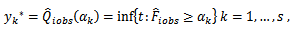
is the customary distribution function estimator based on the sample

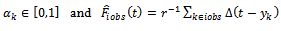
The value is chosen such that the data set after imputation leads to a better overall estimate for the parameters of interest. It seems reasonable to assume that the value could be taken at regular intervals from the cumulative distribution function of variable observed on the sample Taking this consideration into account, we proposed two choices: the first is

(1)

As an example, the proposed imputation method when, given by Eq. (1), use the quartilesfor imputation.

The second choice, according to Munonz and Rueda[14], is

(2)

In the case of Eq. (2) use the minimum, the median and the maximum values

Note that the value of can not exceed the number of observed values for each subject, since this method can be categorized as a hot deck method and, the donors assigned for missing values are taken from respondents in the current sample. Also, only the first missing observation in each subject is imputed. Once, we imputed this value the remaining missing values can be considered as missing completely at random.

After applying the proposed imputation method, we have datasets. Apply the chosen statistical analysis on each of these imputed datasets, for ignorable mechanism. For each pseudo complete data we fit the selection model and obtain the parameter estimates. Fitting selection model mean estimating the parameters in two steps. The first step, the maximum-likelihood estimates of the model parameters are obtained using an appropriate optimization approach. The EM scoring algorithm[21] is used in this paper. In the second step, the maximum-likelihood estimates of the missing data mechanism parameters (the logistic model) are obtained. An iterative maximum-likelihood estimation approach of binary data models, see for example[22], can be used.

Once the analyses have been completed for each imputed data set, we combine these analyses to produce one overall set of estimates. Combining the estimates from the imputed data sets is done using rules established by Rubin[8]. These rules allow the analyst to produce one overall set of estimates like the produced from a non-imputation analysis.

Suppose is the point estimate for a scalar parameter, Rubin's rules specify that combining the estimates of the parameter of interest is accomplished simply by averaging the individual estimates produced by the analysis of each imputed data set. In mathematical terms, this is written generally as:

(3)

for imputed data sets.

In the case of ignorable missing data the Jennrich and Schucher method[21] can be used to obtain maximum likelihood estimates. This is an iterative technique and adopted in this paper.

3.2. Standard Errors of Estimates

We suggest a bootstrap method to obtain the standard errors of the estimates. The bootstrap method was introduced by Efron[23], also in[24], as a computer based method to estimate the standard deviation of the parameters estimates . This approach utilizes resampling from the original data. When the sample size is large, the bootstrapping estimates will converge to the true parameters as the number of repetitions increases.

The basic idea of the bootstrap involves repeated random samples with replacements from the original data. This produces random samples of the same size of the original sample, each of which is known as a bootstrap sample and each provides an estimate of the parameter of interest.A great advantage of bootstrap is simplicity. It is a straightforward way to derive estimates of standard errors and confident-intervals for complex estimators of complex parameters of the distributions, such as percentiles, proportions, and odds ratio, since it is completely automatic, and requires no theoretical calculations. Moreover, it is an appropriate way to control and check the stability of the results.

Generally, bootstrapping follows the same basic steps:

1. Select B independent bootstrap samples each consists of data values drawing with replacement from This create bootstrap data sets of the same size as the original.

2. Apply the estimate procedure to the bootstrap samples by estimating the desired statistic, which forms the sampling distribution of Such that:

3. Estimate the standard error by the sample standard error of the B replicates

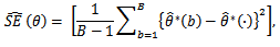with

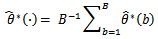Let be the estimated parameter in sample samples, and let be its estimated standard error. The mean of and it's estimated standard error is given by Rubin[8]:

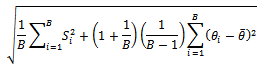In other words, this is the square root of the average of the sampling variances plus the variance of estimates multiplied by a correction factor (Allison[13]).

4. Application (Antidepressant Data)

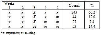
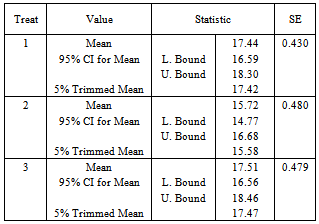
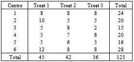
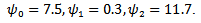
The data represent a multi-centre study of depression. The number of individuals enrolled in the trial is 367 depressed patients from six centres. In each centre, participants were randomly assigned to 3 different treatments. About 20 participants assigned to each treatment in each centre. Each participant was rated on the Hamilton depression score (HAMD). A response scale from 0 to 50, was produced from 16 test items. The HAMD score were expected to take on each participant over 5-weekly visits. The first visit made before treatment, the remaining four during treatment.

Table 1 shows the distribution of unit response pattern over 5 weeks. There were 243 (66.2%) of the participants completed all follow-up assessments. At the termination of the study, up to 124 (33.8%) of the participants had withdrawn from the study.

Table 1. Unit response patterns*

Table 2. Mean Profile of the treatments

Table 2 shows the profile means of each treatment which based on the observed data. The second treatment has the lowest mean profile of a value 15.72. Nevertheless; these means are considered to be biased.

Figure 1 shows the set of measurements for completers at each centre. It can be noticed from the figure the following: first, there is a typical decrease over time of HAMD scores in all centres. Second, the highest rate of variation of the measurements between participants is at week 5. Third, there is a participant in centre two taking treatment 3 who starts and remains at high value.

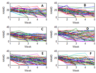Figure 1. Observed measurements of antidepressant data and centers: : (A) center 1; (B) center 2; (c) center 3; (D) center4; (E) center 5; (F) center 6

Table 3 shows number of participants who dropouts at each treatment in each centre. Centre 6 has the highest rate of dropout, regarding the treatment. The highest rate of dropouts occurs at treatment 1. Dropouts occur consistently from week 3 to week five, except in the second treatment in centre 6, all dropouts occur in week 3. Generally, week 3 has the highest number of dropouts.

Table 3. Number of dropouts at centre*treatment combination

Non-random missing data is of particular concern in depression trials because it is very likely that the reason for a participant missing an assessment or dropping out of the study is related to their underlying depression status[11]. For example, a depressed participant may feel that the treatment is not of benefit for him/her and may be unwilling to sit through an interview or any kind of assessment. Conversely, a high-functioning, non-depressed participant may feel that he/she no longer needs to remain in the trial or may not be available for an assessment because he/she is busy with life. Failure to take into account the missing data mechanism may result in inferences that make a treatment appears more or less effective.

We considered two choices of multiple imputation based on quantiles to handle the missing data. Each is based on assuming that the dropout rate is non-ignorable. As mentioned earlier that the dropout occur from week three, and we have five measurements to each participant, i.e. the smallest observed measurements for each subject is two observations. The proposed MI method is considered to be a hot deck procedure; hence we set the number of multiple imputations to be three. We impute the first missing value as we argue that the remaining missing values are missing completely at random. We apply Eq. (1) and Eq. (2) to impute the missing value. In the special cases were the number of observed measurements is two (found in 53 cases (14.4%)), we imputed the missing value with the average of the two observed measurements.

Table 4. The estimates and their standard errors for antidepressant data

The mean profiles are modelled as

(4)

for centre and where giving 8 parameters for the model. The sixth centre and the third treatment are the base categories. The covariance matrix is left unstructured, so there are 15 covariance parameters for the five time points. Other covariance structures can be used. The dropout process is modelled using the logistic model:

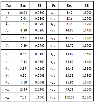
where In this case the underlying dropout rate is set to 0 for the first and second weeks, when there are no dropouts, and constant for weeks 3 - 5.

The proposed strategy is used to obtain the parameter estimates. The results are presented in Table 4. Also, the bootstrap standard errors are presented.

From the results we can see that all the parameters are significant except This means that the first centre effect is not significant and the remaining centres effect is significant. Also, all treatments have significant effects because estimates are significant. The parameters are significant. The parameter is of main interest. This parameter represents the missing not at random process. The significance of this parameter means that the missing data process is missing not at random.

5. Simulation Study

The purpose of this simulation study is to evaluate the performance of the estimates of proposed multiple imputation method. The simulation setup is as follows. The sample size, is chosen to range from small to large. We consider the sample sizes m=20, m= 50 andm=100 to represent small, moderate and, large sample sizes respectively. The number of time points (repeated measures) is fixed at 5. Each subject is allocated randomly to one of two groups; treatment or control group with 50% probability. We use the linear regression model 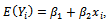where 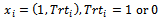indicating treatment or control group. The covariance matrix is left unstructured.

For the missingness model we used the model; where k=3,4,5.

Data are simulated from the multivariate normal model, the unstructured covariance matrix and the missingness model. The parameters values are

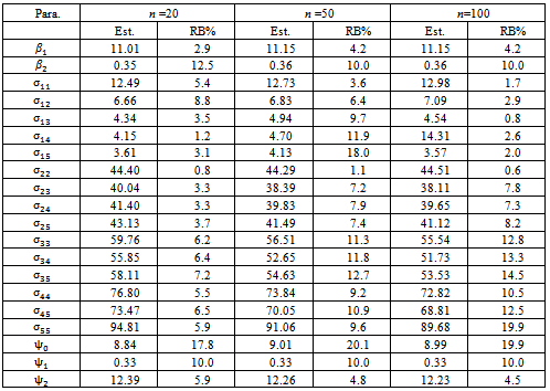
The proposed approach has been applied and then the parameter estimates are obtained. For each simulation we used 10000 replications. The relative bias (RB%) is obtained for each parameter. The simulation results are summarized in Table 5.

From the simulation results we notice that the relative bias of all parameters is below 20% which is reasonable value. This indicates that the proposed technique gives reasonable results for different sample sizes. The relative bias of is around 10% for all sample sizes. This parameter is of main interest because it represents the difference in slope between the two groups.

Other models for the covariance structure have been tried. Also different values formissingness model parameters have been used. The qualitative results are the same as theabove results, so they are not reported.

6. Conclusions

Modelling and analysing the missing values in the longitudinal data context have gained popularity in recent years. Imputation methods are emerged as an aid to such analysis. Multiple imputations is a branch of imputation techniques in which the missing value is replaced by a group of values, resulting in a group of pseudo complete data sets. These data sets are analysed separately and then the overall analysis is obtained. In this paper we present a new multiple imputations strategy based on quantiles. The proposed method is a development of Munoz and Ruedo method to the longitudinal data setting. This method has many advantages; at least it is less biased comparable to other methods. The proposed method is applied in the case of dropout pattern. The method can be easily extended to the intermittent pattern. The selection model[6] is used to fit the data after imputation step. The proposed technique is applied to a real data set.

Table 5. The relative bias of parameter estimates