1. Introduction

Consider a finite population. Let and denote the study variable and an auxiliary variable taking values and respectively on the ith unit. Let, be the population means and be the population variances of and, and be the population covariance between and. Consider a sample of units drawn from according to simple random sampling without replacement (SRSWOR) to estimate the unknown mean. Let and be the sample means,

and the sample variances, and 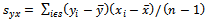be the sample covariance.

The classical regression estimator of that utilizes known value of is defined by 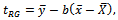where is the familiar least squares estimator of, the population regression coefficient of on. The main advantages associated with are that it can cover both the situations of positive and negative correlations between and, and its precision is usually higher than that of the simple expansion (direct) estimator as well as its ratio and product counterparts. In early days regression estimator was not frequently used in practice because of its computational difficulty. But later on, due to advancement of computational facilities, the regression or regression-type estimators are of much interest to the survey statisticians.

The approximate variance of is given by

(1.1)

where is the correlation coefficient between and. The precision of is usually discussed in terms of. But the exact value of this variance is unknown as it depends on the unknown population quantities and. Hence, the estimation of the variance of seems to be an important aspect of study in the survey sampling literature. An estimate of the variance is needed to provide a measure of the error in estimation of the mean by. A variance estimate is also used to construct a confidence interval for the unknown mean. A commonly used estimator of the approximate variance is its sample analogue

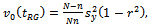(1.2)

where is the sample correlation coefficient, a consistent estimate of.

Survey sampling literature provides a number of procedures for estimating unknown variance using auxiliary information based either on the classical approach [cf., Das and Tripathi[1], Isaki[2], Kadilar and Cingi[3], Grover[4], Yadav[5]] or on the predictive approach [cf., Bolfarine and Zacks[6], Biradar and Singh[7], Nayak and Sahoo[8]]. On the other hand, estimation of correlation coefficient although receives considerable attention in many research papers [cf., Gupta and Singh[9], Shevlyakov[10], Roy[11], Shevlyakov and Smirnov[12]], the sample correlation coefficient still remains as the most discussed estimator of. Hence, our mechanism of estimating in this work consists of selecting alternative estimators of in place of and selecting as the estimator of in the usual way. We assume that both and are known accurately.

2. Formulation of the Estimators

As pointed out earlier, our principal interest here is the estimation of with special concentration on the use of an estimator for that incorporates the available auxiliary information on. This means that we focus attention on the creation of variance estimators having the following generalized form:

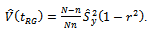(2.1)

This generalized variance estimator can generate a family of estimators of for various selections of. This goal can be achieved by many alternatives ways. But, the variety of finite population variance estimation methods and variety of estimator selection criteria leave us wondering which estimator could be used successfully. The literature to date also offers little guidance in this choice. However, as we are concerned with the variance estimation, we give more stress on the property of non-negativity of an estimator. 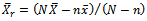It means that we do not consider some estimators of that achieve negative values very frequently under repeated sampling from a given population. Let us now present a brief review of the estimators those are taken into account in the present work.

Two notable but simple estimators under classical approach due to Das and Tripathi[1] and Isaki[2] are very much popular in survey practice. These estimators are defined by

and,

respectively. It may be mentioned here that when, is reduced to the estimator of Deng and Wu[13].

During the years that followed, emphasis has also been given on the prediction of the population variance using auxiliary information. Under this approach, the survey data are at hand i.e., the sample observations are treated as fixed and unassailable. Uncertainty is then attached only to the unobserved values which need to be predicted. To take the advantage of this criterion, the population is decomposed into two mutually exclusive domains and of and units respectively, where denotes the collection of units in which are not included in s. Biradar and Singh[7], Nayak and Sahoo[8] considered the following predictive equation to predict developed earlier by Bolfarine and Zacks[6]:

(2.2)

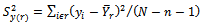where,; and are the implied predictors of and respectively.

For different selections of and, (2.2) can lead to a number of estimators of. But, here we report below six estimators viz., , , suggested by Biradar and Singh [7], and, , suggested by Nayak and Sahoo[8]:

After identifying eight estimators of, we then utilize equation (2.1) to produce estimators of by substituting an estimator for. This operation generates eight estimators corresponding to different but specific choices of as shown in Table 1. To save space, the detail expressions of proposed estimators are not given.

3. Performance of the Proposed Estimators

Generally we judge estimators by their design-based qualities, such as design expectation and design variance, under repeated sampling with a given design from the fixed finite population. The regression estimator is no exception. We are thus interested in evaluating the statistical properties of the eight variance estimators i.e., , compared to the traditional estimator. But, this cannot be done exactly, because of the complex nature of the considered estimators. However, here we rely on a Monte Carlo simulation in which 5000 independent samples for and are drawn from 20 populations available in various text books and research papers on survey sampling. The following performance measures of an estimator are taken into consideration:

(i) Standard Error (SE) : This performance measure of is defined by

,

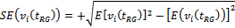which is a convenient and widely used indicator of the precision attained by the variance estimator.

Table 1. Proposed Estimators of

(ii) Coverage Rate (CR) Based on 95% Confidence Interval for Estimating : We consider an approximate 95% confidence interval for based onand its variance estimator defined by under the assumption that sampling distribution of is approximately a normal distribution. This performance measure gives us an idea about which percentage of the so constructed confidence intervals based on the variance estimator covers the true value of under repeated draws of independent samples from a population.

4. Description of the Monte Carlo Simulation

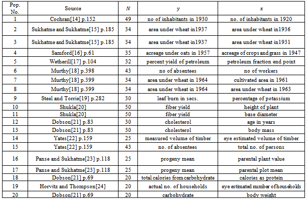
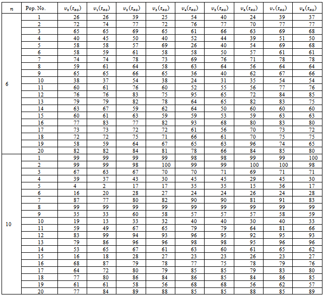
Our Monte Carlo study involves repeated draws of simple random without replacement samples from 20 natural populations. Table 2 presents the source, size, definitions of the variables y and x in respect of these populations. 5,000 independent samples, for and 10, were selected from each population and for each sample numerical values of the comparable estimators were calculated. Then, considering 5,000 such combinations, simulated values of the performance measures viz., SE and CR were computed and summarized in Tables 3 and 4. Results for are not shown, as they confirm more or less the tendencies found in the cases of and 10. Major findings of the study are discussed in subsections 4.1 and 4.2.

4.1. Results Based on the Standard Error

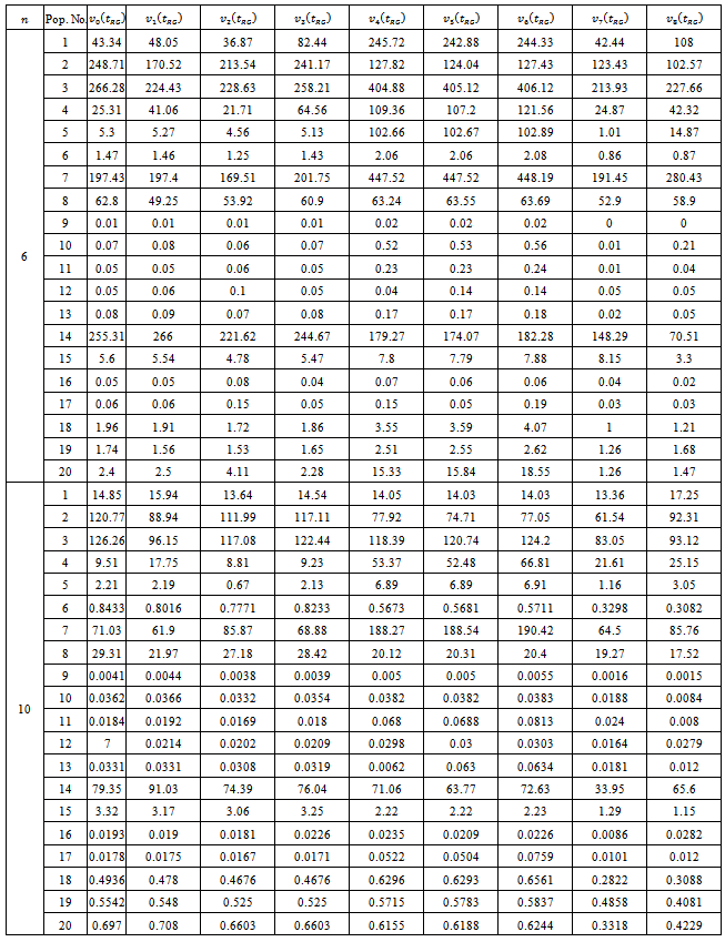
Simulation results on the SE of the different estimators are provided in Table 3. From these results, as is usually expected, we note that the SE of an estimator diminishes with enlargement of sample size. In respect of this criterion, the performance of seems to be very poor, and the estimators behave very much erratically and there is no clear indication that which one of them would have a decidedly better overall performance than other two estimators. The estimator emerged out as the best performer as it is decidedly more efficient than the rest of the estimators in 12 and 9 populations for and 10 respectively, and ranked as second in 6 and 9 populations for and 10 respectively. However, on this consideration we may choose and as the second best and third best performers respectively.

4.2. Results Based on the Coverage Rate

Using several variance estimators, the coverage rates of nominal 95% confidence intervals for are shown in Table 4. The results on the CR give clear indication of improvement in the performance of an estimator as the sample size increases. The CR of the estimators (except some few cases) usually bears no resemblance to the nominal rates aimed at. The three estimatorsperform equally well. However, on the ground of the achieved CR we may consider , and as the best, second best and third best performers respectively.

Table 2. Populations Under Study

Table 3. Standard Error of the Estimators

Table 4. Coverage Rate of the Estimators

5. Conclusions

Our Monte Carlo simulation study shows that the estimator is preferable to its competitors on the grounds of SE and CR. It means that this variance estimator is more efficient than others and can also produce shorter confidence intervals for the population mean. On the other hand, the estimators and may be considered as the second best choice on the consideration of SE and CR respectively.

Although the conclusions of this Monte Carlo investigation may not be applicable to all situations, they provide certain guidelines on the overall performance of the variance estimators under consideration. Further investigations in this direction with the help of other performance measures may be more useful for better understanding of the statistical properties of the estimators.