S. K. Chhillar, S. C. Malik, J. Nandal
Department of Statistics, M.D. University, Rohtak, 124001, Haryana, India
Correspondence to: S. C. Malik, Department of Statistics, M.D. University, Rohtak, 124001, Haryana, India.
| Email: |  |
Copyright © 2012 Scientific & Academic Publishing. All Rights Reserved.
Abstract
An attempt has been made to analyze a single-unit system subject to random shocks. The system may or may not be affected by the impact of shocks. There is a single server who visits the system immediately to conduct maintenance and repair of the unit. The unit undergoes for maintenance if it is affected by the impact of shocks. However, repair of the unit is done when it fails due to some other reasons. The unit works as new after maintenance while it becomes degraded after repair. The degraded unit may work for the system and is replaced by new one giving some replacement time if it is affected by the impact of shocks. Repair of the degraded unit is done if it fails due to the reasons other than shocks. The degraded unit is considered as degraded after repair. The time to failure of the unit and time to occurrence of a shock are exponentially distributed whereas the distributions of maintenance, repair and replacement times are taken as arbitrary with different probability density functions. The expressions for various reliability indices are derived in steady state using semi-Markov process and regenerative point technique. Giving particular values to various costs and parameters, the numerical results are obtained for mean time to system failure (MTSF), availability and profit to depict their graphical behavior with respect to shock rate.
Keywords:
Single-Unit System, Random Shocks, Maintenance, Repair, Degradation, Replacement and Profit Analysis
Cite this paper: S. K. Chhillar, S. C. Malik, J. Nandal, Analysis of a System Reliability Model Subject to Degradation and Random Shocks, International Journal of Statistics and Applications, Vol. 3 No. 3, 2013, pp. 64-70. doi: 10.5923/j.statistics.20130303.05.
1. Introduction
In most of the industrial systems, the method of redundancy has been used to improve their performance and availability. But there are many systems in which a unit cannot be kept as spare due to its high cost. Therefore, stochastic models of single-unit systems with different types of failure and repair policies have been probed by the researchers including Malik and Bansal[1], chander[2] and Malik[3] keeping in view of their practical utility and common man’s affordability. But most of these models have been probed under the common assumptions that failures occur in the system due to reasons other than shocks and system works as new after repair. However, in practice these assumptions are not always true. Since shocks are the events which can be one of the causes of the system failure and deterioration. And, working capacity and efficiency of a failed unit after repair depend more or less on the standard of the repair mechanism exercised. In case of being repaired by an ordinary server, the chances of its failure may be higher and thus such a unit is declared as degraded. Chander and Singh[4] analyzed a 2-out-of-3 redundant system subject to degradation. Wu and Wu[5] obtained reliability of a two-unit cold standby repairable system under Poison shocks. It is also interesting to note that not much work related to the reliability modeling of the single-unit systems subject to random shocks and degradation has been reported so far in the literature of reliability.While considering the above observations and facts in mind, the purpose of the present paper is to analyze a reliability model for a single-unit system subjected to random shocks and degradation. The operative unit may be affected by the impact of shocks with some probability. The unit may fail completely due to the reasons other than shocks. If the unit is affected by the impact of a shock its maintenance is carried out by a server who visits the system immediately. However, repair of the unit is done if it fails due to the reasons other than shocks. The unit works as new after maintenance while it becomes degraded after repair. The degraded unit may work for the system and is replaced by new one giving some replacement time if it is affected by the impact of shocks. Repair of the degraded unit is done if it fails due to the reasons other than shocks. The degraded unit is considered as degraded after repair. The time to failure of the unit and time to occurrence of a shock are exponentially distributed whereas the distributions of maintenance, repair and replacement times are taken as arbitrary with different probability density functions. The expressions for various reliability measures such as transition probabilities, mean sojourn times, mean time to system failure (MTSF), availability, busy period of the server due to repair, replacement and maintenance, expected number of maintenances, expected number of replacements, expected number of repairs and profit function are derived in steady state using semi-Markov process and regenerative point technique. The numerical results for MTSF, availability and profit functions are obtained for a particular case to depict their graphical behavior with respect to shock rate (μ).
2. Notations
E : Set of regenerative states.O : The unit is operative and in normal mode. p0 : The probability that shock is effective.q0 : The probability that shock is not effective.p1 : The probability that degraded unit is affected by the impact of shock.q1 : The probability that degraded unit is not affected by the impact ofshock.µ : Constant shock rate of the unit.λ : Constant failure rate of the unit.λ1 : Constant failure rate of the degraded unit.m(t)/M(t) : pdf / cdf of maintenance time after shock effect. FUr / FWr /FUR : The Unit is completely failed and under repair/waiting for repair/ under repair from previous state SUm/SUM : Shocked unit under maintenance/under maintenance continuouslyfrom previous state SWm : Shocked unit waiting for maintenanceg(t) / G(t) : pdf / cdf of repair time of the completely failed unitf(t) / F(t) : pdf / cdf of replacement time of the degraded failed unitg1(t) / G1(t) : pdf / cdf of repair time of the degraded failed unitqij(t)/ Qij(t) : pdf/cdf of direct transition time from a regenerative state i toa regenerative state j without visiting any other regenerative state. qij.k(t) / Qij.k(t) : pdf/cdf of first passage time from a regenerative state i to a regenerative state j or to a failed state j visiting state k once in (0,t]. Mi(t) : Probability that the system is up initially in state Si  E is up attime t without visiting to any other regenerative state.Wi(t) : Probability that the server is busy in state Si up to time t without making transition to any other regenerative state or returning to the same via one or more non regenerative states.mij : Contribution to mean sojourn time in state Si when system transits directly to state
  where mij =
  = - qij*/(0) and µi is the mean sojourn time in state Si
  E Ⓢ / © : Symbol for Stieltjes convolution / Laplace convolution.~ / * : Symbol for Laplace Stieltjes Transform (LST) /Laplace Transform (LT).‘(desh) : Symbol for derivative of the function.
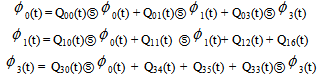
 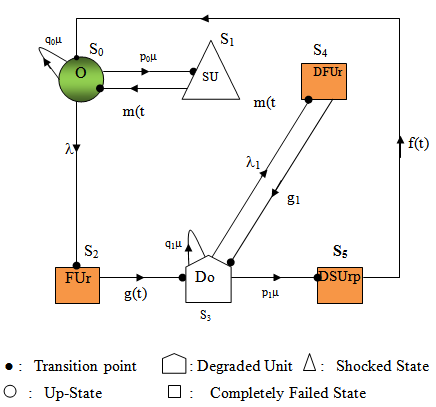 | Figure 1. State Transition Diagram |
The following are the possible transition states of the system S0 = (O), S1 = (SUm), S2 = (FUr), S3=(DO,), S4 =( DFUr),S5=( DSUrp) The transition states S0,S1 and S3 are regenerative and states S2, S4 ,and S5 are non regenerative as shown in figure 1.
3. Transition Probabilities and Mean Sojourn Times
Simple probabilistic considerations yield the following expressions for the non-zero elements as
as
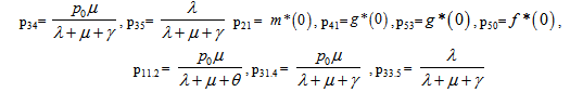 | (1) |
It can be easily verified that | (2) |
The mean sojourn times (i) in the state Si are  | (3) |
For m(t) = 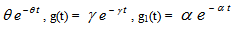 and f(t) =
  we have
 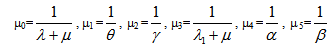 | (4) |
4. Reliability and Mean Time to System Failure
Let  be the cdf of first passage time from regenerative state i to a failed state. Regarding the failed state as absorbing state, we have the following recursive relations for
  :
: | (5) |
Taking L.S.T of above relations (5) and solving for 
 | (6) |
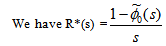
The reliability of the system model can be obtained by taking Laplace inverse transform of (6). The mean time to system failure (MTSF) is given by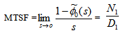 | (7) |
Where

5. Steady State Availability
Let Ai (t) be the probability that the system is in up-state at instant‘t’ given that the system entered regenerative state i at t = 0. The recursive relations for Ai (t) are given as 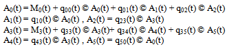 | (8) |
where Mi(t) is the probability that the system is up initially in state  is up at time t without visiting to any other regenerative state, we have
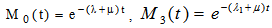 Taking LT of above relations (8) and solving for
  , the steady state availability is given by
 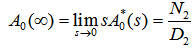 WhereN2 = (1- p33- p34p43) μ0 +p02p23And

6. Busy Period Analysis of the Server
6.1. Due to Repair
Let BRi(t) be the probability that the server is busy in repairing the unit at instant t given that the system entered regenerative state i at t = 0.The recursive relation for BRi(t) are as follows: 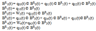 | (9) |
where, 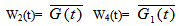 Now taking L.T. of relations (9) and obtain the value of BR0*(s) and by using this, the time for which server is busy in steady state is given by
 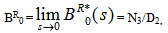 whereN3 = (1- p33- p34p43) q02 W2 + p02p23p34W4 and D2 is already defined.
6.2. Due to Maintenance
Let BMi(t) be the probability that the server is busy in maintenance at instant t given that the system entered regenerative state i at t = 0.The recursive relation for BMi(t) are as follows: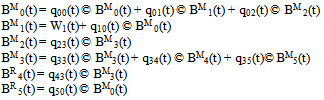 | (10) |
where,  Now taking L.T. of relations (10) and obtain the value of BM0*(s) and by using this, the time for which server is busy in steady state is given by
 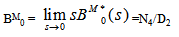 WhereN4 = W1 p01[(1-p33) - p34p43] and D2 is already defined.
6.3. Due to Replacement
Let BRpi(t) be the probability that the server is busy in repairing the unit at instant t given that the system entered regenerative state i at t = 0.The recursive relation for BRpi(t) are as follows: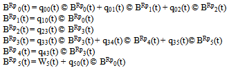 | (11) |
where,  Now taking L.T. of relations (11) and obtain the value of BRp0*(s) and by using this, the time for which server is busy in replacements of the units in steady state is given by
 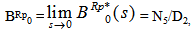 whereN5 = p02p23p35W5 and D2 is already defined.
7. Expected Number of Corrective Maintenance
Let NMi(t) be the expected number of maintenance by the server in (0,t] given that the system entered the regenerative state i at t=0. The recursive relations for NMi(t) are given as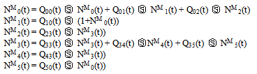 | (12) |
Now taking L.S.T. of relations (12) and solving for NM0*(s) and by using this, the expected number of maintenances by the server is given by 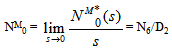 whereN6 = (p10p01)[(1-p33)-p34p43] and D2 is already defined.
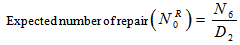
8. Expected Number of Repairs
Let NRi(t) be the expected number of repairs by the server in (0,t] given that the system entered the regenerative state i at t=0. The recursive relations for NRi(t) are given as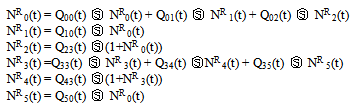 | (13) |
Now taking L.S.T. of relations (13) and solving for NR0*(s) and by using this, the expected number of repairs by the server in steady state is given by 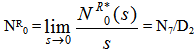 whereN7 = (p02p23)(1- p33) and D2 is already defined.
9. Expected Number of Replacement
Let NRpi(t) be the expected number of replacements by the server in (0,t] given that the system entered the regenerative state i at t=0. The recursive relations for NRpi(t) are given as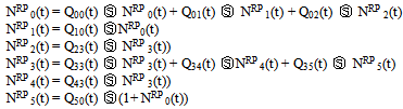 | (14) |
Now taking L.S.T. of relations (14) and solving for NRp0*(s) and by using this, the expected number of replacements by the server in steady state is given by 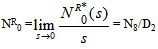 whereN8 = p02p23p35p50 and D2 is already defined.
10. Profit Analysis
The profit incurred to the system model in steady state can be obtained as | (15) |
whereK0 = Revenue per unit up-time of the systemK1 = Cost per unit time for which server is busy due to maintenanceK2 = Cost per unit time for which server is busy due to repairK3 = Maintenance cost per unit K4 = Repair cost per unit K5 = fixed cost of the server and  are already defined.
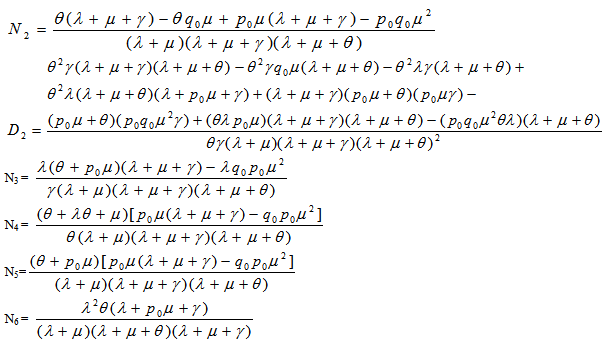
11. Particular Case
Suppose 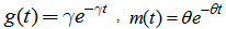 We can obtain the following results MTSF (T0) =
 , Availability (A0) =
  Busy period due to repair
  Busy period due to corrective maintenance
  Expected number of corrective maintenance
 | (16) |
where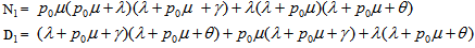
12. Conclusions
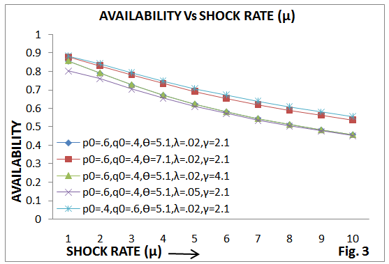
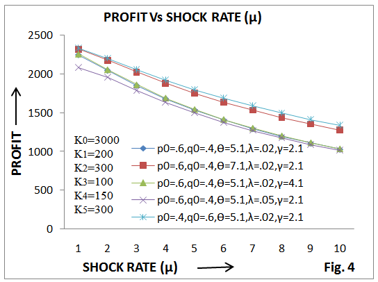
The study reveals that mean time to system failure (MTSF), availability and profit of a single-unit system go on decreasing with the increase of shock rate (µ) and failure rate (λ) for fixed values of other parameters and costs as shown in figures 2, 3 and 4. However, their values go on increasing with the increase of maintenance and repair rates. It is interesting to note that MTSF decreases by interchanging p0 and q0, i.e., p0=.4 and q0= .6 while availability and profit increase. Hence, it is concluded that a single- unit system subjected to random shocks can be made more profitable and reliable to use either by increasing the maintenance rate of the shocked unit or by making replacement of the degraded unit after the impact of shock. 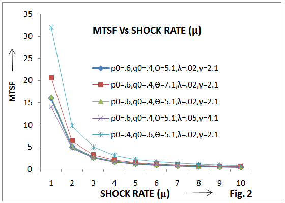 | Figure 2. MTSF Vs. Shock Rate |
 | Figure 3. Availability Vs. Shock Rate |
 | Figure 4. Profit Vs. Shock Rate |
References
| [1] | Chander, S. and Bansal, R.K. (2005): Profit analysis of single-unit reliability models with repair at different failure modes, Proc. INCRESE IIT Kharagpur, India, pp. 577-587. |
| [2] | Chander, S. (2007): Profit analysis of reliability models with priority in operation as well as in repair, Statistical Techniques in Life Testing, Reliability, Sampling theory and Quality Control, Narosa Publishing House, New Delhi, pp. 153 – 162. |
| [3] | Malik, S.C. (2008): Reliability modeling and profit analysis of a single-unit system with inspection by a server who appears and disappears randomly, Journal of Pure and Applied Mathematika Sciences, Vol. LXVII, No. 1-2, pp. 135-146. |
| [4] | Malik, S.C. and Singh, M. (2009): Probabilistic analysis of 2-out-of-3 redundant system subject to degradation, Journal of Applied Probability and Statistics (USA), Vol. 4(1), pp. 33 – 44. |
| [5] | Wu, Q. and Wu, S. (2011): Reliability analysis of a two-unit cold standby reparable systems under Poison shocks. Applied Mathematics and Computation, Vol. 218 (1), pp. 171-182. |
 Abstract
 Reference
 Full-Text PDF
 Full-text HTML