1. Introduction

Human societies are often stratified into classes on the basis of things such as income, occupation, social status or place of residence. Members of such societies move from one class to another in what often seems to be a haphazard manner. In the field of social stratification attention is increasingly turned to the facts concerning mobility. For example, sons do not always follow in their fathers’ footsteps and even if they do, the varying members of offspring in different classes would lead to fluctuations in the class sizes. Similarly, in a free society, a person has some degree of choice to change his job or to change his house. Again, the inherent uncertainty of individual behaviour in these situations means that the future development of the mobility process cannot be predicted with certainty but only in terms of probability. So, as probability is there, it would be suitable to apply a stochastic model whose essential ingredient is to give a probabilistic description of any particular situation or any particular phenomena. Thus, any stochastic model of mobility can give a probabilistic description of how movement takes place from one class to another. Here, in this paper, in the simplest type of model, the assumption is made that the chance of moving depends only on the present class and not on the past.

There are very many processes in the natural and social sciences which can be represented as a set of flows of objects or people between categories of some kind. The Markov chain model has been used in the study of many of some kind. Anderson[2] and Miller[3] attempted to describe changes in voting behaviour as a Markov Process. The earliest paper in which social mobility was viewed as a stochastic process appears to be that of Praise[1]. More work is covered by Cheng and Jianzhong[4], Hodge[5], McGinnis[6], Henry and co-workers[7], Henry[8], Spilerman[9], Krishnan and Sangadasa[10]. More recently Beller and Hout[11] examine trends in US social mobility, especially as it relates to the degree to which a person’s income or occupation depends on his or her parent’s background. Social class is always defined in terms of occupation. The pioneering study in this field of social mobility is by Blumen and co-workers[12], whose ‘mover-stayer’ model occupies a central place in his paper. Wyrn and Sales applied this model to the British Labour Force.

The important two applications which have received particular attention are the closely related fields of social and occupational mobility. A society is divided into classes on the basis of social status or occupation and the changing structure of society is studied with the aid of the model. So, in this paper, an effort is made to focus on the social mobility by using the celebrated Markov chain model.

A number of empirical studies of mobility have been published which give sufficient data to provide a partial test of the theory. One of these due to Glass and Hall[13] is based on a random sample of 3500 pairs of fathers and sons in Britain. They had classified the members of their sample according to the seven occupational groups. A second study made by Rogoff[14] is based on data from marriage licence applications in Marion County, Indiana. Rogoff obtained data for two periods; one from 1905 to 1912 with a sample size of 10253 and a second from 1938 to 1941 when sample size was 9892. Moreover data relating to Denmark are given in Svalagosta. Praise applied this model to the data obtained by Glass and Hall[13]. This work is also carried out in the lines of the works of Praise[1].

As discussed by the earlier authors that the concept of social mobility is complex; its study is best furthered by the kind of quantitative approach so widely adopted. This, again, is in accord with views expressed in earlier investigations such as that of Ginsberg[15], Praise[1]. Perhaps the most interesting table of statistics resulting from such quantitative studies is one setting out the relation between the social statuses of fathers and their sons as derived from a series of interviews of a sample of population. Here in this paper such a table is given below as Table1 and will be termed as a transition matrix; for the elements of which will be regarded as estimated probability of a family’s transition from one social class to another. The matrix is based on the results of a random sample of some 4798 male, residents in Golaghat in the state of Assam, India and over interviewed during the period November 2011 to August 2012. Here, in this paper, it is tried to study about the mobility structure regionally than nationwide. As to know about all over the country, it is recommended to study regionally before.

Moreover here it is assumed that these probabilities are constant over time[16] and with the help of this assumption a number of new summary measure will be derived seem to have advantages over those currently used in assessing the degree of social mobility[17].

One important point, however, in interpreting the calculation given below is that ‘social class’ has been treated as if it is related only to the male side of the family line; this is largely because social class has in this study been measured by occupation. One more assumption made in the present analysis is that the influence of one’s progenitors in determining one’s class is transmitted entirely through one’s father, so that if the influence of one’s father has been taken into account, then the total influence of one’s progenitors is accounted for.

2. Methodology Adopted

2.1. The Basic Model

First we consider a very simple model for the development of a single family line. The fundamental requirement in a model is that it must specify the way in which chances in social class occur. We shall assume that these are governed by transition probabilities which are independent of time. Let denote the probability that the son of a father in class ‘i’ is in class ‘j’; since the system is closed

where k is the number of classes.

If we consider only family lines in which each father has exactly one son, the class history of the family will be a Markov chain. But in practice, the requirement that each father shall have exactly one son is not met. However for a stable population, each father will have an average one son. We may expect our results for the simple model to apply in an average sense in such an actual society.

2.2. The Equilibrium Distribution of the Social Class

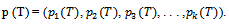
Suppose that the probability that the initial progenitor of a family line is in class ‘j’ at time zero is . Let the probability that the line is in class j at time T (T=1, 2, 3, ...) be . The probabilities can then be computed recursively from the fact that

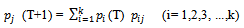(2.2.1)

In matrix notation these equations may be written as

(2.2.2)

where The unit of time implied in this equation is a generation.

Repeated application of (2.2.2) gives

(2.2.3)

The elements of p(T) may also be interpreted as the expected proportions of the population in the various classes at time T. If the original classes of the family line are known, the vector p(0) would then represent the initial class structure.

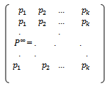
The matrix plays a fundamental role in the theory of Markov Chains. It can be used to obtain the ‘state probabilities’ from (2.2.3), but its elements also have a direct probabilistic interpretation.

In many applications the population has been in existence for many generations so that the ‘present’ state corresponds to a large value of T. It is therefore required to investigate the behaviour of the probabilities as T tends to infinity. It is shown in the general theory of Markov chain that this limiting behaviour depends on the structure of the matrix P. Provided that the matrix P is regular, it may be shown that these probabilities all approach limits as T tends to infinity. A regular (finite) Markov chain is one in which it is possible to be in any state (class) after some number, T, of generations, no matter what the initial state. More precisely, a necessary and sufficient condition for some the chain to be regular is that all of the elements of are non-zero for some T.

With the existence of the limits assured it is a straightforward matter to calculate them. Thus if we write 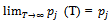it follows from (2.2.2) that the limiting structure must satisfy

(2.2.4)

with

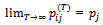
An important property of the solution is that it does not depend on the initial state of the system. Since, by our assumptions, each family line extant will have reached the equilibrium given by (2.2.4), the vector p gives the expected structure of the population at the present time. The limiting value of , denoted by , can be deduced from (2.2.3). It must satisfy

(2.2.5)

which can only be so if

(2.2.6)

which implies that

(2.2.7)

The foregoing analysis shows that if our model provides an adequate description of actual societies then their future development depends only on their initial structure and the transition matrix. Of these two features the initial distribution has a diminishing influence as time passes. In the long run, therefore, the structure of the society is determined by its transition matrix. From this point, we may imply that the study of mobility must be centred upon the transition probabilities. In particular, measures of mobility should be functions of the elements of P.

2.3. The Average Time Spent in a Social Class

The average number of generations spent in a social class is most simply calculated as follows:

Let there be families in class ‘i’ in the current generation. Of these the number will be found in the class in the next generation; the number will be found in the third generation and so on. Hence, the total time spent in the class by the families at present in that class is

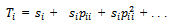On dividing by there results the average time, , spent by a family in that class; thus

(2.3.1)

And Standard Deviation (SD) of the time spent in each social class can be shown to be as:

(2.3.2)

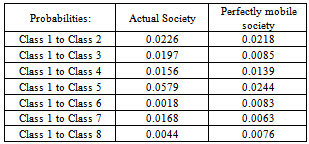
In order to use the measures in assessments of the mobility of a society it is necessary to know what would be the corresponding values of these measures in a society that is perfectly mobile. This can be defined as:

In terms of the transition matrix, a perfectly mobile society is a society in which the probability of entering a particular social class is independent of the class of one’s father; so that all the elements in each row of the matrix would be substantially equal (to any given degree of approximation), though there would generally be difference between the rows. A more general definition of perfect mobility would make the probability on entering a class substantially independent of that of one’s progenitor; where the first progenitor is defined as the father, the second progenitor as the grandfather and so on.

2.4. The Variation of Mobility with Time

The measure of mobility given in the last section is of a particularly simple sort it depends only on the amount of self-recruitment in each class- that is, on the diagonal elements of the transition matrix. The other elements only enter into the calculation of the equilibrium distribution which is used as a standardized factor.

In this section a set of rather more complicated measures is proposed which have the advantage that it is possible to assess with their aid the amount of movement among the various social classes achieved in successive generations; these measures depend more directly on all the elements of the matrix. They arise from the observation that in societies such as those described by Table1 not only is the degree of self-recruitment higher than in a perfectly mobile society, but also the degree of recruitment from adjacent classes is higher than that from the more distant classes.

The generalisation to great grandsons,great-great-grandsons and so on, to yield Immobility Factors for the third generation, fourth generation and so on, is now straightforward. The possibility of doing this is considerably simplified by the theorem as given below in this section which holds for any perfect mobile society.

Suppose that M denote the number of family lines in the population; this remains constant through time. The numbers of family lines in the class were enumerated now and, after an interval of n generations, they were enumerated again. At the second generation it would be found that a certain proportion, say , of those family lines originally in the class were still in that class. The theorem states that in a perfectly mobile society this proportion does not depend on the number of intervening generations; that is is independent of T.

The proof of this proposition, if needed, is simple. For the proportions are the elements of a matrix defined by an equation analogous to equation (2.2.3). Now, if M is the transitions matrix of any perfectly mobile society that is, for all i and k it is true that then the elements of are given by

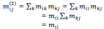Since the sum of any row is unity. Hence,

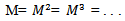And, in particular,

(2.5.1)

On the other hand, in a society that is at all immobile, the ratio of family lines to be found in the class now to those who were originally in that class T generations ago (and have either stayed in that class for the intervening T generations or have left that class and returned to it) will depend on the value of T (so long as T is finite). The ratios will in fact be given by the diagonal elements, , of the matrix defined in equation (2.2.3) above. The measures of immobility for the generation are then defined as

3. Results and Discussion

It is convenient to begin by setting out the transition matrix used as the basis for all the subsequent calculations in this paper. It is given in Table1. The element of row of this matrix, to be denoted by , gives the proportion of fathers in the social class whose sons move into the social class; alternatively, if it is supposed that there is some unambiguous method of tracing the family line through time, then represents the probability of a transition by a family from class i into class j in the interval of one generation.

Here in this study, the different types of occupations are gathered into broad classes as given below so that a matrix can be created and which allows comparing each person’s occupation with his father’s occupation.

The states, that is, the occupational classes or the social classes that are used in our investigation are described as:

1. Professionals: (Scientists, engineers, doctors, accountants, lawyers, lecturers and teachers, actors, reporters, Police, electrician, drivers)

2. Managers and Administrators: (Managers in banks, tea gardens, Administrator in national and local government, party organization)

3. Clerical workers: (Clerks, secretaries, Post office workers)

4. Agricultural workers: (Workers in agriculture, forestry, husbandry, Fishing)

5. Self employed: (Individual workers, private entrepreneurs)

6. Sales workers: (Shop assistants, salesmen)

7. Manual workers: (Manual workers in manufacturing, Construction, transport)

8. Personal service workers: (Waiters, ushers, stewards, nannies, hairdressers, Cleaners)

That is; i, j = 1, 2, 3,..., 8.

If the table is taken a column at a time, the elements show how the probabilities of entering a given class vary with the class of one’s father. Since everyone must be in some class (whatever the class of one’s father) it follows that the sum of each row is unity.

Adequacy of the Model:

The equilibrium distribution is also independent of the unit of time in which the elements of P are measured; suppose, for example, that observations were taken to allow the writing of an equation similar to (2.2.1) showing the relationship between the social statuses of grandson and grandfather. Every element of the transition matrix would then be different since it would refer to a transition during a period of two generations instead of one generation. The equilibrium distribution corresponding to such a matrix would however be unchanged. For, if the matrix relating the statuses of fathers to sons is P, that relating those of grandsons will be P² and when these matrices are raised to the power, they obviously tend to the same value as n tends to infinity.

Table 1. The Estimated Social Transition Matrix in Golaghat

Table 2. Actual and Equilibrium Distribution of the Social Classes in Golaghat

The first two columns of Table2 give the actual distribution of the classes, as estimated from the sample observations, for the sons and for the fathers (two succeeding generations). If the Markov model is adequate and if the society has reached equilibrium we would expect these distributions to be the same, apart from sampling fluctuations. We would also expect them both to agree with the equilibrium distribution obtained from (2.2.4). In this paper, the calculations necessary for this comparison and the results are given in column (3) in Table 2 and from the results it has been observed that the distributions are remarkably similar and hence even if the transition matrix of Table1 continues to hold entirely unchanged over the next few generations, no great changes are to be expected in the distribution of the population among the various social classes.

A more precise comparison of the results is made in the last column (4) of the table2 which shows the ratio of the proportion of the current generation that is of the sons in each class to the proportion to be expected in equilibrium.

The Average Time spent in a Social Class:

The results of the calculations based on the formulae given above[equation (2.3.1) and (2.3.2)] are set out in Table3.

Table 3. The Average Number of Generations spent in each Social Class in Golaghat

The first column shows that even when only eight groups are distinguished in the population, in no case does the average number of generations spent by a family in a particular social class exceed two. The longest time is 1.62 generations for the professional class. The impression that families may spend longer than this in a particular class is no doubt due to the wide dispersion of the actual times; as will be seen from column (4) of the table 3, the standard deviations are in fact considerable.

The second column of the table3 shows the average number of generations that would be spent in each class if the society were perfectly mobile. The least time 1.04, 1.05 and 1.06 generations would be spent in the managerial, sales workers and personal service workers class; whereas 1.36 generation is spent by the professional class.

The measures of the immobility structure of the social structure are given in column (3). From the column (3), it is observed that the social classes: clerical workers, personal service workers, manual workers and sales workers are affected approximately equally, but not much, by the effects of immobility; while the social classes: professional and managerial are affected quite high by the immobility and the figure for the social class agricultural workers seem excessive when compared to the others.

Referring to Table1 it may be seen that the probability of moving from class 1 to Class 2 in the first generation (0.0599), and then back into Class 1 in the second generation (0.3779), is given by the value 0.0599 × 0.3779 = 0.0226. On the other hand, the probability of moving from Class 1 to the distant Class6 (0.0176) and back again (0.1051) is given by the much smaller value of 0.0176 × 0.1051 = 0.0018. In the similar but perfectly mobile society (based on the equilibrium values given in Table 2) the value of these probabilities would be, respectively, 0.2629 × 0.0828= 0.0218 and 0.2629 × 0.0459 = 0.0083. All the probabilities from the Class 1 to other Classes for the actual society along with the perfectly mobile society are given as in Table 4:

Table 4. Probabilities from class1 to other classes in Actual and Perfectly Mobile Society

The computed probabilities of Table4 reveal that: for the actual society, the probability from the class professional to the classes: sales workers and personal service workers are lower as compared to the other classes. On the other hand, the probability of return to the professional class from self employed class is much higher than the other classes. Similarly, for the perfectly mobile society; the lowest probabilities range from 0.0063 to 0.0085 for the classes: manual workers, personal service workers, sales workers and clerical workers and the highest probability is 0.0244 for the class self employed.

The net effect, that is, the probability of moving into any other class from the class1 (professional class) and then back into that class1 may be found by summing over the seven classes and will be found to have the value 0.1388 as compared with the value of 0.0908 to be found in perfectly mobile society. If the probability of self recruitment is included in these figures, as is especially convenient when these measures are generalised to ‘n’ generations, these results the probability of finding one’s grandson in one’s own class irrespective of whether one’s son has remained in the same class or not. The values obtained for the class1 in the actual and perfect mobile society are then 0.2844 and 0.2629. The ratio of these two figures is 1.08 and may be termed the Immobility Factor for the second generation relating to the first class.

The immobility ratios for the first to the fourth generations in Golaghat are given below:

Table 5. Immobility Ratios for the First to the Fourth Generations in Golaghat

First, for t=1, this measure has a direct relationship with the measure based on the average time spent in each class which was considered in the last section. However, it is not possible from knowledge of one of these measures alone to obtain the other.

Secondly, as t becomes larger, the Immobility Ratios for all classes tend to unity, indicating that after a sufficiently long time the number of descendants to be found in one’s own class differs arbitrarily little from that to be found in a perfectly mobile society.

Immobility ratios for the first five generations have been calculated from the data given in Table1 and the results are brought together in Table5. The data shows that in the first generation there is a fair amount of mobility: the largest index is that for the class agricultural workers 7.83; and the lowest value is that for the personal service workers class 0.67 where there is a negligible amount even of the first generation immobility.

By the time the third generation is reached all the classes except the agricultural workers class may be judged to be fully mobile for practical purpose. The index shows, however, that the agricultural class has three times as many great grandsons in its own group than would be found in a perfectly mobile society. Even by the time the fourth generation is reached, the index for this class is still higher than that for the other classes. On the other hand, from the indices of the classes: managerial, clerical, sales and manual workers it may be interpreted that these classes will have less numbers of great-grandsons in their own group than would be in a perfectly mobile society; specially, the personal service workers class will have very less number of great-grandsons in its own class than in a perfectly mobile society.

The idea to be gained from this table as to the extent of social immobility, and its importance as a factor in social policy, may at first sight be quite different from that gained from the previous table from which it is appeared that, on the average, the time spent in any social class did not exceed two generations. It is, therefore, worth adding that the two sets of measures are entirely consistent apart from the agricultural workers class.

4. Conclusions

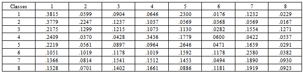
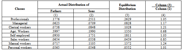
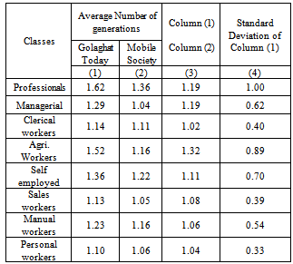
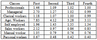
From the Table1, we have observed that probability of sons being in professional class is 0.3815 when their fathers were in the same class. Similarly, the probability of sons being in managerial class is 0.2274 when their fathers were in the same class. Similar interpretations can be made for the other classes also.

Table 2 gives the class structure of the population in two succeeding generations. On the whole, it has been observed that the probabilities for the sons increase as compared to the fathers for all the classes except the classes: agricultural workers, sales workers and personal service workers, that is, the low level classes. Also, if the transition matrix of Table1 continues to remain unchanged over the next few generations, no noticeable changes are to be expected in the distribution of the population among the various social classes.

Again, the last column of the Table2 gives a more precise comparison on the ratio of the proportion of the current generation, i.e., of the sons, in each class to the proportion to be expected in equilibrium. The figures indicate that if the recruitment to the various classes proceeds as it has in the past generations then the proportion in the classes: professional, managerial, clerical, self employed manual and personal service workers will rise, while the proportion in the classes: agricultural workers and sales workers will decline to some extent.

From the calculations of Table3 (column 1), we have seen that no family lines can spend average number of generations in any social class exceeding two, maximum being 1.62 and minimum 1.10.

From the second column of Table3, which gives the average number of generations that would be spent in each social class for perfectly mobile society; we have observed that almost all the social classes would spend about only one generation if the society would be perfectly mobile.

The third column of the table3 indicates that the agricultural workers following professional and managerial class are affected much by immobility factor. The net result for the respective social classes are about 32 per cent, 19 per cent and 19 per cent respectively; that is, the average family lines spend between 19 per cent to 32 per cent more time in the social classes mentioned above than if the society were completely mobile. However, for the other classes the average family lines spend between 2 per cent to 11 per cent more time than in a perfectly mobile society.

From Table4, we have observed that from the class professional the probability of moving into the class self employed and back to that class is high; and the probability to the class personal service workers class and back to his own class are very low.

The Table5 reveals that the agricultural workers class has three times more great- grandsons in its own class and the class personal service workers will have very less numbers of great-grandsons in its own class than would be found in a perfectly mobile society.

ACKNOWLEDGEMENTS

It is a pleasure to acknowledge the help and valuable suggestions which I have received in preparing this paper to Dr. S.C. Kakaty, Professor, Department of Statistics, Dibrugarh University. Also, I would like to offer my sincere thanks to all the inhabitants of Golaghat, Assam for providing me the required data.