Muhammad Nur Aidi M.S1, Tuti Purwaningsih S.Stat2
1Department of Statistics, Faculty of Mathematics and Science, Bogor Agricultural University, Dramaga, Bogor, West Java, 16680, Indonesia,
2Master Student at Department of Statistics, Faculty of Mathematics and Science, Bogor Agricultural University, Dramaga, Bogor, West Java, 16680, Indonesia
Correspondence to: Muhammad Nur Aidi M.S, Department of Statistics, Faculty of Mathematics and Science, Bogor Agricultural University, Dramaga, Bogor, West Java, 16680, Indonesia,.
| Email: |  |
Copyright © 2012 Scientific & Academic Publishing. All Rights Reserved.
Abstract
This study is intended to determine the factors that affect poverty-stricken districts in Java Island by using spatial ordinal logistic regression (SOLR). This study is urgent for local governments since they have a mission for the welfare of their citizens, especially alleviating poverty that occurred in each region. The evaluation is based on the best model and to evaluate SOLR model with and without handling multicollinearity. The principal component (PC) is for handling multicollinearity. This research used secondary data (Kusumaningrum, 2010)[6]. Results showed the ordinal logistic regression (OLR) model with all explanatory variables spatial has Correct Classification Rate (CCR) value of 50%. Then the OLR with PC model has a CCR of 24%. So it can be concluded that SOLR model is better than OLR with PC model. Based on spatial model without PC, there are five variables that influence the level of district poverty on Java island, namely: the number of farmers, small industries, families without electricity, hospitals and spatial variable on districts poverty. The variables that have negative correlation are the number of farmers, families without electricity and spatial variables. Increase in the number of farmers and families without electricity will reduce the chances of a district becoming rich. The spatial correlation is negative, which means that if a district is surrounded by districts with high poverty levels, the chances of a district to become more wealthy will decline.
Keywords:
Spatial Ordinal Logistic Regression, Handling Multicollinearity, The Principal Component Analysis, Poverty, CCR.
Cite this paper: Muhammad Nur Aidi M.S, Tuti Purwaningsih S.Stat, Modeling Spatial Ordinal Logistic Regression and The Principal Component to Predict Poverty Status of Districts in Java Island, International Journal of Statistics and Applications, Vol. 3 No. 1, 2013, pp. 1-8. doi: 10.5923/j.statistics.20130301.01.
1. Introduction
1.1. Background
Java Island is the most populous island in Indonesia. Java Island consists of 6 provinces namely the Special Capital Region of Jakarta, West Java, Banten, Central Java, Yogyakarta and East Java. Each province consists of several districts.Each province has its vision and mission for the welfare of its citizens, especially in terms of alleviating poverty that occurred in each region. Fund available for this program is limited, so it is necessary to have an election as to which district is entitled as an object of this program. One way is to categorize districts into 6 levels of poverty so that the funds can be assigned on a priority scale. Poverty status of a district cannot be separated from the influence of the status of poverty in the surrounding district. This indicates the existence of spatial effects. Pratama (2008)[9] and Thaib (2008)[11] perform spatial modeling logistics against poverty status of a region. Both studies concluded that the estimation of poverty of an area using spatial logistic regression will yield a better prediction than the classical logistic regression. Logistic regression model with the categorization of spatial poverty into two categories: poor and non-poor has been done by Suprapti (2009)[10]. Therefore, in this research, we use ordinal logistic regression model spatially for six categories.
1.2. Purpose
The purpose of this research is to know the factors that affect poverty-stricken districts in Java based on Spatial ordinal logistic regression model and to evaluate spatial ordinal logistic regression with and without handling multicollinearity.
2. Review Literatures
2.1. Poverty
Indonesia is a developing country with the majority of the population experiencing poverty problem. In general, poverty is a situation where there is an inability to meet basic needs such as food, clothing, shelter, education and health. There are several definitions of poverty made by government and non government agencies. According to the Statistics Center a household is poor if it has a per capita income below the poverty line. The poverty line is the minimum size of one's income that can still be used to meet basic human needs. Meanwhile, the World Bank defines extreme poverty as a condition in which a person lives on less than U.S. $ 1 per day and poverty if someone has an income of less than U.S. $ 2 a day. Pre-Prosperous Family is a family that cannot meet the minimum standards of basic human needs such as spiritual needs, food, clothing, housing, education and health. Prosperous families are families that can afford to meet basic human needs, but cannot meet higher human needs (BKKBN 2004)[3]
2.2. Ordinal Logistic Regression
Ordinal logistic regression was used to model the relationship between variables with ordinal-scale response variables with explanatory variables. If the response variable Y is assumed there is an ordinal scale with K categories and x= (x 1, x 2, ..., x p) is the vector of explanatory variables, then the chances of the variable response of the k-th category of explanatory variables X in particular can be expressed by P  and the cumulative odds is in Function 1 (Hosmer & Lemeshow 2000)[5].
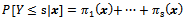 | (1) |
Cumulative logit model is defined by Function 2.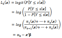 | (2) |
where  and
and  is the threshold model and
  is a vector of regression coefficients.Parameter estimation method that can be used in ordinal logistic regression is the Maximum Likelihood method. This method can be done if the observations are assumed to be independent. Its likelihood function for a sample with n independent observations, (yi, xi), i = 1,2, ..., n, can be expressed as follows in Function 3 (Hosmer & Lemeshow 2000)[5]
 | (3) |
 While the log likelihood function defined in Function 4 below.
 | (4) |
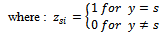
Furthermore, to obtain estimators of parameters of the ordinal logistic regression function is to maximize the log likelihood of parameters.In ordinal regression analysis there are five options for liaison function (link function) as found in Table 1. Their use depends on the distribution of the analyzed data. Logit is used in most data distribution. Complementary log-log is used for data that have a tendency of high value. Negative log-log is used for data that have a tendency of low-value, while probit is used if the spread is normally latent variables, whereas cauchit (Cauchy inverse) is used if latent variables have extreme values. Ordinal regression analysis previously described is an ordinal regression analysis with logit link function often called the ordinal logistic regression (Norusis 2010)[8].Table 1. Function Liaison Ordinal Regression
 |
| |
|
2.2.1. Significance Testing Model
Likelihood ratio test of the model used to estimate the parameters with the hypothesis: H1 : there is at least one
 , where i is the number of explanatory variables.Likelihood ratio test statistic uses the G, where G = -2 ln (L 0 / L k) where L 0 is the Likelihood function without variables and L k is the Likelihood function with variables (Hosmer & Lemeshow 2000)[5]. If H 0 is true, Statistics G will follow a Chi-square distribution with degrees of freedom p and Ho will be rejected if the value of G> X2(p, α) or p-value <α. Wald test is used to test the significance of each coefficient in the model. The hypothesis is:
 H1:
H1:  , where i is the number of explanatory variables.Wald test calculates a W statistic, defined as
 Reject H 0 if | W |> Z α / 2 or p-value <α (Hosmer & Lemeshow 2000)[5].
2.2.2. Assumptions of Logistic Regression
Logistic regression has the following assumptions (Garson 2010)[4]: The data has no outliers. In logistic regression, outliers can affect the results significantly. It is recommended that there should be no multicollinearity among the explanatory variables.
2.2.3. Interpretation of Logistic Regression
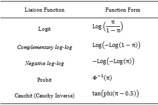
Interpretation for ordinal logistic regression model can be done using the odds ratio value. Suppose for a nominal-scale variables X(x 1 and x2), the odds ratio in the category Y ≤ s is defined in Function 5 (Agresti 1990)[1] and Dillon and Goldstein (1984)[3].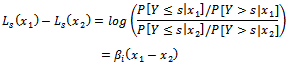 | (5) |
With i = 1, 2, …, p (p = number of explanatory variables) and s = 1, 2, …, S-1. βi is coefficient logistic regression2) with meaning is: 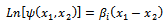 So we get estimators for the odds ratio
  as follows (Agresti 1990) )[1]:
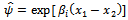 For categorical explanatory variables, if the odds ratio value is > 1,then the odds x1 is greater than the odds x2 or in other words,
  will always be greater than
  . So it can be said, when x 1 chance for
  greater than at x 2.For the continuous explanatory variables, x, the odds as x increases one unit is equal to
  multiply odds when x has not increased. If the value of the odds ratio > 1, then probablity for
  is greater when x be increased than x has not increased. For large-scale continuous variables, required a change of c units to interpretation, with an odds ratio of
  .
.
2.3. Spatial Analysis
Spatial analysis is an analysis which includes the influence of spatial or space into the analysis. In spatial analysis the correlation between spaces is called spatial correlation. Thus each observation is not free stochastic (Ward & Gleditsch 2008)[12].The types of spatial data are data points, data line, polygon data and latis data. Data points are divided into discrete points and continuous point. Line data are for example, road maps, river or coastlines. Polygon data for example is a map of a garden in terms of irregular shapes. The latis data is for example provinces in which there were districts.
2.3.1. Contiguity Matrix
Contiguity matrix is a matrix that describes the relationship between regions, giving the value 1 if the area i neighbor with area j, while a value of 0 is given if area i is not adjacent to the area-j. Lee and Wong (2001)[7] refer to this matrix as binary matrix, and also called the connectivity matrix, which is denoted by C, and c ij being the value of matrix in row i and column j. Later in this study, it will be referred to as matrix W containing w ij for row i and column j.
2.3.2. Spatial Ordinal Logistic Regression
Spatial Ordinal Logistic Regression is an analysis which incorporates spatial effects into the ordinal logistic regression model. Suprapti (2009)[10] uses spatial logistic regression model of the form: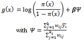 Where is a form of auto-covariance and is a weighted average of the number of events among the k i neighbors. Weighting of the location of the ij-th is through w ij= 1 / h ij where h ij is the euclid distance between the village i and j.
  is the alleged existence of an event. Another model which could be established to handle the spatial relationships is :
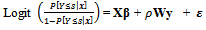 Where k is a category sth from all of the dependent variables and W is a weighting matrix that represents the spatial proximity of the region. w ij = 0 if regions i and j are not adjacent regions directly while w ij = 1 if regions i and j areas are immediately adjacent. Spatial weighting matrix (W) which has been obtained is multiplied by the vector y and the results will be considered as new variables and will be used in ordinal logistic regression analysis. In general, the parameter estimation process includes the testing of hypotheses, drawing conclusions and interpretations, following the rules in ordinal logistic regression
2.4. Model of Validation
Validation of models is using the Correct Classification Rate (CCR). CCR is the percentage of correct observations (suitability with the expected value). CCR can be calculated using the following Function 6: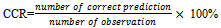 | ....(6) |
The higher percentage of CCR shows higher accuracy (Hosmer and Lemeshow 2000)[5].
2.5. Winsorizing Methods
Winsorizing method is one method to handling outliers, without having to lose the observation data. This method is particularly suitable for modeling data in which observations should not be eliminated. In this method the outliers are replaced with a value closest to it.
3. Materials dan Methods
3.1. Material
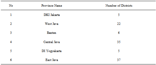
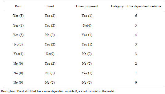
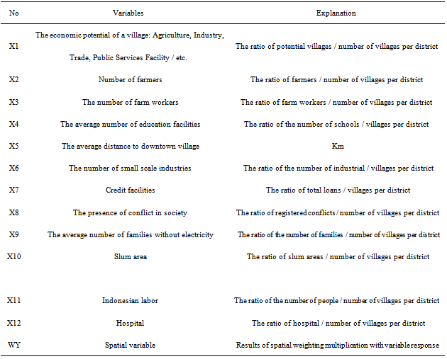
Data used in this research is secondary data obtained from hotspot poverty districts data in Java which is obtained from the research by Kusumaningrum (2010)[6].Dependent variables used in this study are presented in Table 3.Explanatory variables used in this study are presented in Table 4.Table 2. List of Number of Districts
 |
| |
|
Table 3. Ordinal Scale Poverty
 |
| |
|
Table 4. List of Variables
 |
| |
|
3.2. Method
To achieve the objectives of this research, namely: a) To know the factors that affect poverty-stricken districts in Java based on ordinal logistic regression models of spatial. It can be done by the following procedures:• Selection of explanatory variables that will be used in the analysis, by looking at the closeness of the relationship of these variables. • Response variables to be used is a hotspot poverty districts in the island of Java in the form of ordinal data with 6 categories from research that has been done by Kusumaningrum (2010)[6].• Looking at the closeness between districts in Java.• Creating a spatial weighting matrix W which contains 1 if adjacent, and 0 if not directly adjacent.• Create a new variable result multiplication of matrix W` with Y, namely X spatial (WY)• Checking the assumption of logistic regression• Forming ordinal logistic regression model that has incorporated the spatial variables X using 100% data.• Identifying whether the coefficient of X spatial is significant or not. If significant, indicate whether the spatial correlation influences poverty. Then identify the significance of the other X variables.• Getting the ordinal logistic regression model with spatial variable X that is significant. b)To evaluate the spatial ordinal logistic regression model of ordinal logistic regression model. It can be done by following these procedures:• Estimating the value of the dependent variable with ordinal logistic regression using 100% spatial data. In this case, do not cross validate because this model does not aim to predict the level of poverty from a new emerging district.• Measuring the value of CCR from spatial ordinal logistic regression model then comparing with the value of CCR results from ordinal logistic regression model. A higher CCR value indicates that the model has better accuracy.
4. Results and Discussion
4.1. Exploration Data
The data in this study consisted of one response variable in the form of district poverty level category, and 14 explanatory variables. Poverty Distribution Category of the districts with the respective percentages can be seen in Figure 1. The highest percentage occurs in poverty level category 5, meaning that poor districts are experiencing problems and insufficient food and that is as much as 33.3% of all districts in Java. While the number of districts with the lowest category 1 means that only the district experiencing the problem of unemployment.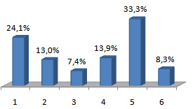 | Figure 1. Percentage of district poverty category |
4.2. Test of Logistic Regression Assumptions
4.2.1. Detecting Outliers and Handling
Logistic regression analysis assumes that the data has no outliers, then the prior is modeled, while outliers are treated before hand with Winsorized Mean method. Sample distribution of data containing outliers can be seen in Figure 2. Once resolved, the results can be seen in Figure 3. 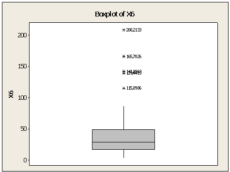 | Figure 2. Examples of data contained outliers |
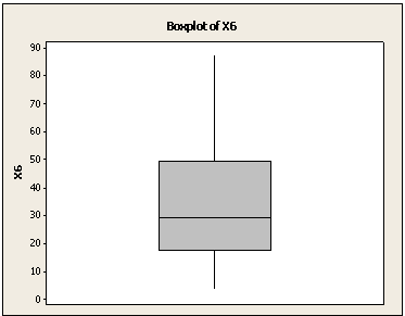 | Figure 3. Example of the data after outliers corrected |
4.2.2. Detecting Multicollinearity and Handling
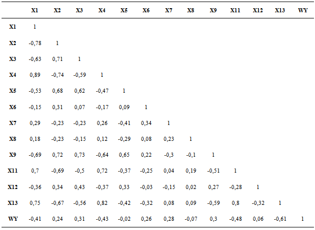
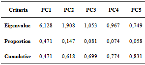
Explanatory variables are correlated with each other resulting in so-called multicollinearity. In logistic regression, there must be no multicollinearity because in the presence of multicollinearity the standard error of regression coefficient will be increased so that the possible results of Wald test of each X will not be significant. However, this assumption is actually not very important because multicollinearity does not change its estimate value.To select the best model, we compute CCR. So we must compare the results of the CCR with the handling of multicollinearity and the results of the CCR without handling multicollinearity.The value of correlation between explanatory variables can be seen in Table 5. The values show that some variables are correlated highly enough and some quite low. Multicollinearity is handled by using principal components analysis. The 13 explanatory variables were reduced into 3 main components, namely PC1, PC2 and PC3. The process of determining the number of components be used if total of CCR is greater than 70%.Principal component analysis results can be seen in Table 6.Table 5. The Correlation between Explanatory Variables
 |
| |
|
Table 6. Principle Components
 |
| |
|
4.3. Spatial Ordinal logistic Regression Using The Principal Component Analysis
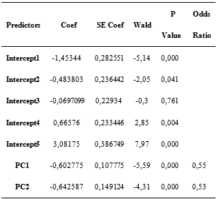
After building a model for ordinal logistic regression with 3 main components, it is known that only the first and second components are significant of influence on the response variable, with a given level of diversity of more than 60%. The result can be seen in Table 7, as follows:Table 7. Ordinal Logistic Regression Model with Main Components
 |
| |
|
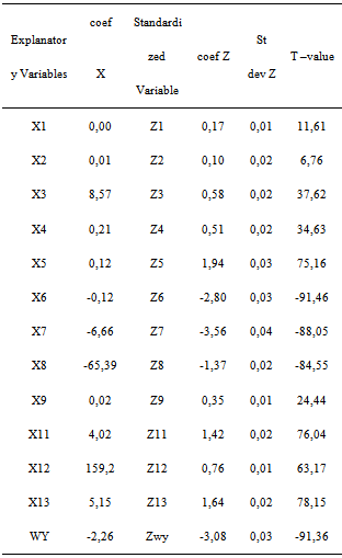
After learning that the only PC1 and PC2 are significant influence, transformation of the PC towards explanatory variables namely X1, X2 ..., X13 and WY is carried out. The result can be seen in Table 8 below.Table 8. Results of inverse transformation
 |
| |
|
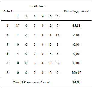
Table 8 shows that all the variable X has a T value count greater than 1.96 which means that all explanatory variables influence the level of poverty in the district under 5% significance level (also significant at 15% significance level). The CCR value of this model is then calculated. The result can be seen in Table 9.Table 9. CCR Spatial Ordinal Logistic Regression Model with Principal Component
 |
| |
|
Based on table 9, the result Correct Classification Rate, is small enough, almost 24%.This shows that this model is less good based on the expected value of 14 explanatory variables. Therefore it is necessary in further study that all explanatory variables are included in order to have a model that is really quite good in classifying district poverty category. Furthermore, ordinal logistic regression modeling was developed using the entire spatial explanatory variables.
4.4. Spatial Ordinal Logistic Regression Models without Handling Multicollinearity
4.4.1. Modelling
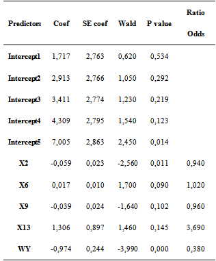
In this section, a model of spatial ordinal logistic regression is made by including all explanatory variables, without reducing it into a major component. The result can be seen in Table 10.Table 10. Spatial Ordinal Logistic Regression Models with all explanatory variables
 |
| |
|
4.4.2. Evaluation of Spatial Ordinal Logistic Regression Models
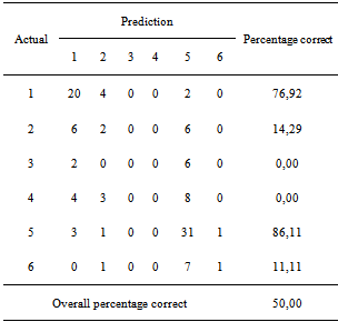
Evaluation models can be made by using the likelihood-ratio test using the statistical G. Based on the analysis, G = 81.485 with p = 0.000 indicates that Ho was rejected, meaning that there is one explanatory variable that significantly influence the level of poverty of a district. Further evaluation is to use measure of association, Correct Classification Rate (CCR) and the Goodness of fit test which will be described further below.In measuring association, the values of concordant and discordant couples show how good a model is to predict the data. Concordant value of 81% shows that as many as 81% of districts with poverty rates (<k) have better chance in predicting the category (<k). While the value of discordant 18.7% indicates that as many as 18.7% districts with poverty rates (> k) have a better chance predicting the category (<k). This means that the size of the association in this model is very good. Table 11. CCR Spatial Ordinal Logistic Regression Models with All Explanatory Variables
 |
| |
|
Table 11 shows that the CCR of spatial ordinal logistic regression model is 50%. This means that 50% of the districts are predicting correctly through the model. The test Goodness of Fit using Chi Square yields a value of 464.904 with the value of p of 0.965. Therefore, the spatial logistic regression model has good model fit.
4.4.3. Factors Determining the Impact of Poverty Level
Based on Table 10, it can be seen that the model with no treatment of multicollinearity is better than that with the handling of multicollinearity, because it has a higher CCR value. The conclusion derived is that ordinal logistic regression model without the handling of spatial multicollinearity was used as a reference model to see the variables that influence the level of poverty. Based on the above explanation, an increase in the number of farmers, the number of families who do not have electricity on a county to reduce the chances of a district to be poor. Meanwhile, by increasing the average number of small industries and the number of hospitals to increase the chances of a district to be poor.
4.4.4. Identifying the Spatial Variable
Looking at the spatial variables (WY), one can say that there is spatial correlation between district poverty levels and this can cause the poverty of a district to influence neighboring districts. Then after further examined, variable spatial relationship with poverty rates assumes a negative value, This means districts with lower levels of poverty are usually surrounded by districts with high poverty level.
4.5. Comparring Spatial Model with and without Handling Multicollinearity
By comparing the value of CCR, we can say that spatial ordinal logistic regression model is better than the principal component regression because it has higher CCR value that is equal to 50%, while with the principal component model has a CCR value of 24%. Therefore, in this case, handling multicollinearity with principal component is the good choice.
5. Conclusions and Suggestions
5.1. Conclusions
Increasing of the number of farmers, the number of families who do not have electricity on a county to reduce the chances of a district to be poor. Meanwhile, by increasing the average number of small industries and the number of hospitals to increase the chances of a district to be poor. Based on the analysis that has been done, it can be concluded that there are five variables that affect poverty-stricken districts in Java namely: the number of farmers, the number of families who do not have electricity in a district, the percentage of slum area in a district, the average number small industries, the number of hospitals and the district spatial poverty variable. Therefore, these factors should be prioritized in reducing poverty levels in all districts on the island of Java.
5.2. Suggestion
Based on these results, it is suggested that attention is given to the value of CCR at the time of logistic regression modeling. There is a need for further study regarding the degree of influence of multicollinearity on the results of classification, perhaps by creating a simulation. Last but not least, poverty-stricken districts on Java island are advised to consider the factors that affect poverty district.
References
| [1] | Agresti A. Categorical Data Analysis. New Jersey: John Wiley and Sons. USA. 1990. |
| [2] | [BKKBN] National Disaster Coordinating Agency. Family income; Glance.[link] http://www.bkkbn.go.id/article_detail.php[2 October 2011]. 2004. |
| [3] | Dillon, W R and Goldstein, M. Multivariate Analysis. John Wiley & Sons, New York. USA. 1984. |
| [4] | Garson, GD. Logistic Regression.[link] http://www. chass.ncsu.edu[1 October 2012] |
| [5] | Hosmer, DW and Lemeshow, S. Applied Logistic Regression Second Edition. New York : John Wiley and Sons. USA. 2000. |
| [6] | Kusumaningrum D. Hotspot Analysis on Poverty, Unemployment, and Food Security in Java, Indonesia. Thesis. Bogor Agricultural University. Indonesia 2010. |
| [7] | Lee J, and Wong, DWS. Statistical Analysis ArchView GIS. New York: John Wiley & Sons, Inc. 2001. |
| [8] | Norusis, MJ. SPSS Statistics Guides: Ordinal Regression.http://www.norusis.com/pdf/ASPC_ v13.pdf [25 December 2011]. 2010. |
| [9] | Pratama, V. Comparison of Prediction Results of Spatial Regression Model for Different Variogram Models. Thesis. Bogor Agricultural University. Indonesia. 2008. |
| [10] | Suprapti. Weighted distance and optimum Intersection Spatial Logistic Regression for Prediction of Rural Poverty Status in West Java. Thesis. Bogor Agricultural University. Indonesia. 2009 |
| [11] | Thaib, Z. Logistic Regression Modeling Spatial Contiguity Matrix Approach. Thesis. Bogor Agricultural University. Indonesia. 2008 |
| [12] | Ward, MD and Gleditsch, KS. Spatial Regression Models. Los Angeles: Sage Publications, Inc. 2008. |
 Abstract
 Reference
 Full-Text PDF
 Full-text HTML