Navid Feroze 1, Muhammad Aslam 2
1Department of Mathematics and Statistics, Allama Iqbal Open University, Islamabad, Pakistan
2Department of Statistics, Quaid-i-Azam University, Islamabad, Pakistan
Correspondence to: Navid Feroze , Department of Mathematics and Statistics, Allama Iqbal Open University, Islamabad, Pakistan.
| Email: |  |
Copyright © 2012 Scientific & Academic Publishing. All Rights Reserved.
Abstract
In this paper, the problem of estimating the scale parameter of log gamma distribution under Bayesian and maximum likelihood framework has been addressed. The uniform and Jeffreys priors have been assumed for posterior analysis. The Bayes estimators and associated risks have been derived under five different loss functions. The credible intervals and highest posterior density intervals have been constructed under each prior. A simulation study has been carried out to illustrate the numerical applications of the results and to compare the performance of different estimators. The purpose is to compare the performance of the estimators based on Bayesian and maximum likelihood frameworks. The performance of different Bayes estimators has also been compared using five different loss functions. The study indicated that for estimation of the said parameter, the Bayesian estimation can be preferred over maximum likelihood estimation. While in case of the Bayesian estimation, the entropy loss function under Jeffreys can effectively be employed.
Keywords:
Loss Functions, Posterior Distribution, Credible Intervals
Cite this paper:
Navid Feroze , Muhammad Aslam , "A Note on Bayesian and Maximum Likelihood Estimation of Scale Parameter of Log Gamma Distribution", International Journal of Statistics and Applications, Vol. 2 No. 5, 2012, pp. 73-79. doi: 10.5923/j.statistics.20120205.05.
1. Introduction
The log gamma distribution is often used to model the distribution of rate of claims in insurance. Balakrishnan and Chand[1] discussed the best linear unbiased estimators of the location and scale parameters of log-gamma distribution based on general Type-II censored samples. Chung and Kang[2] used the generalized log-gamma distribution to fit the industrial and medical lifetime data. To overcome the Bayesian computation, the Markov Chain Monte Carlo (MCMC) method was employed. Ergashev[3] estimated the lognormal-gamma distribution by using the Markov chain Monte Carlo method and imposing prior assumptions about the model’s unknown parameters. Demirhan andHamurkaroglu[4] proposed a new generalized multivariate log-gamma distribution. The use of the suggested distribution under Bayesian approach has also been discussed. Kumar and Shukla[5] obtained the maximum likelihood estimates of the two parameters of a generalized gamma distribution directly by solving the likelihood equations as well as by reparametrizing the model. Shawky and Bakoban[6] derived Bayesian and non-Bayesian estimators of the shape parameter, reliability and failure rate functions in the case of complete and type-II censored samples. The mean square errors of the estimates have been computed. Comparisons have been made between these estimators using a Monte Carlo simulation study. Chen and Lio[7] studied the maximum likelihood estimates for the parameters of the generalized Gamma distribution using progressively type-II censored sample. Singh et al.[8] proposed Bayes estimators of the parameter of the exponentiated gamma distribution and associated reliability function under general entropy and squared error loss functions for a censored sample. The proposed estimators have been compared with the corresponding maximum likelihood estimators through their simulated risks. Feroze and Aslam[9] considered the Bayesian analysis of Gumbel type II distribution under different loss functions using doubly type II censored samples. The applicability of the results has been discussed under a simulation study. Fabrizi and Trivisano[10] investigated the performance of Bayes estimators of parameter of log-normal distribution using quadratic expected loss. Amin[11] considered the maximum likelihood estimation procedure for estimation of the parameters of the mixed generalized Rayleigh distribution under type I censored samples. Numerical example has been used to illustrate the theoretical results. Dey[12] considered the Bayesian estimation of generalized exponential distribution under different loss functions.In the following sections, the point and interval estimates have derived under maximum likelihood and Bayesian approach. The variances/risks of the point estimators have also been obtained.
2. The Maximum Likelihood Estimation
The maximum likelihood estimator along with its variance has been derived in the following.The probability density function of log gamma distribution is: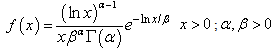 | (1) |
The likelihood function for a sample of size n is: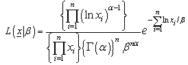 | (2) |
The maximum likelihood estimator of the parameter  and corresponding variance are:

3. Bayesian Estimation under the Assumption of Uniform Prior
For estimation the parameter(s) under a Bayesian framework, it mandatory to decide about an appropriate prior. There is no rule of thumb to select a particular prior; however Berger[13] suggested that even an inappropriate choice of prior can give useful results. In practice the informative priors are not always available, for such situations, the use of non-informative priors become popular. One of the most widely used non-informative priors, due to Laplace[14], is a uniform prior. Therefore, the uniform prior has been assumed for the estimation of the scale parameter of the log gamma distribution. The uniform prior is assumed to be:  The posterior distribution for
  given data under the assumption of uniform prior is:
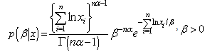 | (3) |
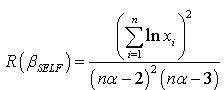
The Bayes estimator and risk under uniform prior using squared error loss function (SELF) are:
 The Bayes estimator and risk under uniform prior using quadratic loss function (QLF) are:
 The Bayes estimator and risk under uniform prior using weighted loss function (WLF) are:
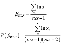 The Bayes estimator and risk under uniform prior using precautionary loss function (PLF) are:
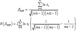 The Bayes estimator and risk under uniform prior using entropy loss function (ELF) are:
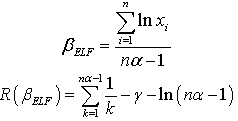 Where is an Euler constant.The Bayes estimator and risk under uniform prior using weighted balanced loss function (WELF) are:
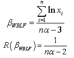
4. Bayesian Estimation under the Assumption of Jeffreys Prior
As discussed in the above section, in case of unavailability of the informative priors the non-informative priors are used. Another non-informative prior has been suggested by Jeffreys[15] which is frequently used in situations where one does not have much information about the parameters. This is defined as the distribution of the parameters proportional to the square root of the determinants of the Fisher information matrix i.e. 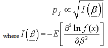 The Jeffreys prior for scale parameter of log gamma distribution is:Here
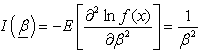
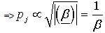 | (4) |
The posterior distribution for  given data under the assumption of Jeffreys prior is:
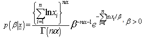 | (5) |
The Bayes estimator and risk under Jeffreys prior using squared error loss function (SELF) are: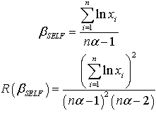 The Bayes estimator and risk under Jeffreys prior using quadratic loss function (QLF) are:
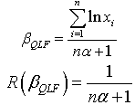 The Bayes estimator and risk under Jeffreys prior using weighted loss function (WLF) are:
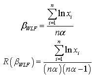 The Bayes estimator and risk under Jeffreys prior using precautionary loss function (PLF) are:
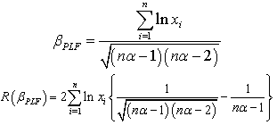 The Bayes estimator and risk under Jeffreys prior using entropy loss function (ELF) are:
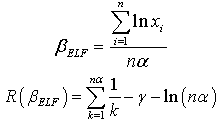 The Bayes estimator and risk under Jeffreys prior using weighted balanced loss function (WBLF) are:
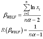
5. The Credible and Highest Posterior Density Intervals
As discussed by Saleem and Aslam[16], the  credible intervals have been constructed under the assumption of uniform and Jeffreys prior and presented respectively.
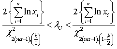
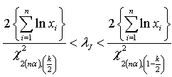 Where
Where  is the confidence coefficient.An interval
  will said to be
  highest posterior density interval for
  if it satisfies the following two conditions simultaneously.
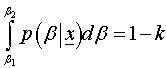 Where
Where  is the confidence coefficient.And
 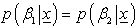 So, the highest posterior density interval for
  under uniform can be obtained by solving the following two equations simultaneously:
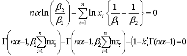 Where
Where 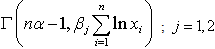 is an incomplete gamma function.Similarly, the highest posterior density interval for
  under Jeffreys can be obtained by solving the following two equations simultaneously:
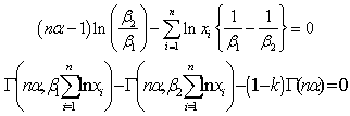
6. The Posterior Predictive Distributions
The posterior predictive distribution is defined as: 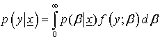 The posterior predictive distribution using the posterior distribution under uniform prior is:
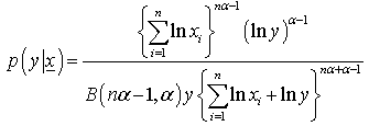 | (6) |
Where  is a beta function.Similarly, the posterior predictive distribution using the posterior distribution under Jeffreys prior is:
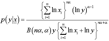 | (7) |
| Table 1. ML and Bayes (under uniform prior) estimates along with their variances for β = 2 |
| | n | MLE | Loss Functions | | SELF | QLF | WLF | PLF | ELF | WBLF | | 50 | 2.143383 | 2.187126 | 2.143383 | 2.165033 | 2.198371 | 2.165033 | 2.209673 | | (0.045941) | (0.049315) | (0.010000) | (0.022092) | (0.022490) | (0.004947) | (0.010204) | | 100 | 2.057927 | 2.078714 | 2.057927 | 2.068268 | 2.083983 | 2.068268 | 2.089266 | | (0.021175) | (0.021934) | (0.005000) | (0.010446) | (0.010538) | (0.002516) | (0.005051) | | 200 | 2.036242 | 2.046474 | 2.036242 | 2.041345 | 2.049050 | 2.041345 | 2.051629 | | (0.010366) | (0.010549) | (0.002500) | (0.005129) | (0.005152) | (0.001258) | (0.002513) | | 300 | 2.022447 | 2.029211 | 2.022447 | 2.025823 | 2.030910 | 2.025823 | 2.032610 | | (0.006817) | (0.006897) | (0.001667) | (0.003388) | (0.003398) | (0.000840) | (0.001672) | | 500 | 1.996488 | 2.000489 | 1.996488 | 1.998486 | 2.001492 | 1.998486 | 2.002495 | | (0.003986) | (0.004014) | (0.001000) | (0.002002) | (0.002006) | (0.000506) | (0.001002) |
|
|
| Table 2. ML and Bayes (under uniform prior) estimates along with their variances for β = 4 |
| | n | MLE | Loss Functions | | SELF | QLF | WLF | PLF | ELF | WBLF | | 50 | 4.293970 | 4.381602 | 4.293970 | 4.337343 | 4.404130 | 4.337343 | 4.426773 | | (0.184382) | (0.197922) | (0.010000) | (0.044259) | (0.045055) | (0.004947) | (0.010204) | | 100 | 4.305496 | 4.348986 | 4.305496 | 4.327132 | 4.360010 | 4.327132 | 4.371062 | | (0.092686) | (0.096009) | (0.005000) | (0.021854) | (0.022048) | (0.002516) | (0.005051) | | 200 | 4.244293 | 4.265621 | 4.244293 | 4.254930 | 4.270990 | 4.254930 | 4.276365 | | (0.045035) | (0.045833) | (0.002500) | (0.010691) | (0.010738) | (0.001258) | (0.002513) | | 300 | 4.132408 | 4.146229 | 4.132408 | 4.139307 | 4.149700 | 4.139307 | 4.153174 | | (0.028461) | (0.028796) | (0.001667) | (0.006922) | (0.006942) | (0.000840) | (0.001672) | | 500 | 4.014124 | 4.022168 | 4.014124 | 4.018142 | 4.024185 | 4.018142 | 4.026203 | | (0.016113) | (0.016227) | (0.001000) | (0.004026) | (0.004033) | (0.000506) | (0.001002) |
|
|
| Table 3. ML and Bayes (under Jeffreys prior) estimates along with their variances for β = 2 |
| | n | MLE | Loss Functions | | SELF | QLF | WLF | PLF | ELF | WBLF | | 50 | 2.143383 | 2.165033 | 2.143383 | 2.143383 | 2.176051 | 2.143383 | 2.187126 | | (0.045941) | (0.047830) | (0.009901) | (0.021650) | (0.022036) | (0.004997) | (0.010101) | | 100 | 2.057927 | 2.068268 | 2.057927 | 2.057927 | 2.073485 | 2.057927 | 2.078714 | | (0.021175) | (0.021605) | (0.004975) | (0.010341) | (0.010433) | (0.002504) | (0.005025) | | 200 | 2.036242 | 2.041345 | 2.036242 | 2.036242 | 2.043908 | 2.036242 | 2.046474 | | (0.010366) | (0.010470) | (0.002494) | (0.005103) | (0.005126) | (0.001255) | (0.002506) | | 300 | 2.022447 | 2.025823 | 2.022447 | 2.022447 | 2.027517 | 2.022447 | 2.029211 | | (0.006817) | (0.006863) | (0.001664) | (0.003376) | (0.003386) | (0.000839) | (0.001669) | | 500 | 1.996488 | 1.998486 | 1.996488 | 1.996488 | 1.999487 | 1.996488 | 2.000489 | | (0.003986) | (0.004002) | (0.000999) | (0.001998) | (0.002002) | (0.000506) | (0.001001) |
|
|
| Table 4. ML and Bayes (under Jeffreys prior) estimates along with their variances for β = 4 |
| | n | MLE | Loss Functions | | SELF | QLF | WLF | PLF | ELF | WBLF | | 50 | 4.293970 | 4.337343 | 4.293970 | 4.293970 | 4.359417 | 4.293970 | 4.381602 | | (0.184382) | (0.191965) | (0.009901) | (0.043373) | (0.044146) | (0.004997) | (0.010101) | | 100 | 4.305496 | 4.327132 | 4.305496 | 4.305496 | 4.338045 | 4.305496 | 4.348986 | | (0.092686) | (0.094566) | (0.004975) | (0.021636) | (0.021827) | (0.002504) | (0.005025) | | 200 | 4.244293 | 4.254930 | 4.244293 | 4.244293 | 4.260272 | 4.244293 | 4.265621 | | (0.045035) | (0.045489) | (0.002494) | (0.010637) | (0.010684) | (0.001255) | (0.002506) | | 300 | 4.132408 | 4.139307 | 4.132408 | 4.132408 | 4.142767 | 4.132408 | 4.146229 | | (0.028461) | (0.028652) | (0.001664) | (0.006899) | (0.006919) | (0.000839) | (0.001669) | | 500 | 4.014124 | 4.018142 | 4.014124 | 4.014124 | 4.020155 | 4.014124 | 4.022168 | | (0.016113) | (0.016178) | (0.000999) | (0.004018) | (0.004025) | (0.000506) | (0.001001) |
|
|
| Table 5. 95% credible intervals under uniform and Jeffreys priors for β = 2 |
| | n | Uniform Prior | Jeffreys Prior | | LL | UL | UL–LL | LL | UL | UL–LL | | 50 | 1.778313 | 2.634314 | 0.856001 | 1.793191 | 2.667094 | 0.873903 | | 100 | 1.800048 | 2.375797 | 0.575749 | 1.807955 | 2.389590 | 0.581635 | | 200 | 1.850551 | 2.251506 | 0.400955 | 1.854765 | 2.257747 | 0.402982 | | 300 | 1.882030 | 2.178076 | 0.296046 | 1.884954 | 2.181993 | 0.297039 | | 500 | 1.910943 | 2.085914 | 0.174971 | 1.912774 | 2.088095 | 0.175321 |
|
|
| Table 6. 95% credible intervals under uniform and Jeffreys priors for β = 4 |
| | n | Uniform Prior | Jeffreys Prior | | LL | UL | UL–LL | LL | UL | UL–LL | | 50 | 3.562603 | 5.277481 | 1.714878 | 3.592409 | 5.343151 | 1.750743 | | 100 | 3.765974 | 4.970528 | 1.204555 | 3.782516 | 4.999386 | 1.216870 | | 200 | 3.857242 | 4.692983 | 0.835740 | 3.866026 | 4.705992 | 0.839965 | | 300 | 3.845499 | 4.450401 | 0.604902 | 3.851472 | 4.458403 | 0.606931 | | 500 | 3.842129 | 4.193924 | 0.351795 | 3.845810 | 4.198310 | 0.352500 |
|
|
7. Simulation Study
Simulation is a technique that can be used to examine the performance of different estimation procedures. In this technique random samples are generated in such a way that estimators under different estimation procedure can be compared and are in accordance with the real life problem. Here, the inverse transformation method of simulation is used to compare the performance of different estimators. The study has been carried out for n = 50, 100, 200, 300 and 500 using  . The risks of Bayes estimates have been presented in the parenthesis. It is immediate from the Tables 1-4 that the estimated value of the parameter converges to the true value as the sample size increases. While the magnitude of posterior risks decreases by increasing the sample size. However, the increase in value of the parameter imposes a negative impact on the rate of convergence and the performance (in terms of posterior risks) of the estimates. The estimates under Jeffreys prior seem to work better than those under uniform prior for each loss function except entropy loss function. Among loss functions the performance of the estimates under entropy loss function is the best. It can also be indicated that with an exception estimates under squared error loss function, the estimates using Bayesian framework provide better results than maximum likelihood estimates.The results of interval estimation are in accordance with the point estimation, that is, the width of credible interval is inversely proportional to sample size while, it is directly proportional to the parametric value. Similarly, the width of credible interval is narrower under the assumption of Jeffreys prior.
8. Conclusions
The study has been conducted to discuss the problem of estimating the scale parameter of log gamma distribution under maximum likelihood and Bayesian framework. It has been assessed that the performance of the Bayes estimation is better than maximum likelihood estimation with some exceptions. In comparison of priors, the performance of the Jeffreys prior is found to be better with an exception of estimates under entropy loss function. Similarly, the estimates under entropy loss function are associated with the minimum risks and the magnitude of these risks is independent of choice of parametric values. The Bayesian interval estimation further strengthens the findings of the point estimation. So, in order to estimate the scale parameter of the log gamma distribution, the Bayesian estimation can be preferred over maximum likelihood estimation. While under the Bayesian estimation, the entropy loss function can effectively be employed.
ACKNOWLWDGEMENTS
Bundle of thanks to referees for their precious suggestions to improve the quality of the paper.
References
| [1] | N. Balakrishnan and P. S. Chand, “Asymptotic Best Linear Unbiased Estimation For The Log-GammaDistribution”, Sankhya : The Indian Journal of Statistics, vol. 56, pp. 314-322, 1994. |
| [2] | Y. Chung and Y. Kang, “Bayesian Analysis in Generalized Log-Gamma Censored Regression Model”, The Korean Communications in Statistics, vol.5, no.3, pp. 733-742, 1998. |
| [3] | B. Ergashev, “Estimating the Lognormal-Gamma Model of Operational Risk Using the Markov Chain Monte Carlo Method”, The Journal of Operational Risk, vo.4, no.1, pp. 35-57, 2009. |
| [4] | H. Demirhan and C. Hamurkaroglu, “On a Multivariate Log-Gamma Distribution and the Use of the Distribution in the Bayesian Analysis”, Journal of Statistical Planning and Inference, vol.141, pp. 1141-1152, 2011. |
| [5] | V. Kumar and G. Shukla, “Maximum Likelihood Estimation in Generalized Gamma Type Model”. Journal of Reliability and Statistical Studies, vol.3, no.1, pp.43-51, 2010. |
| [6] | A. I. Shawky and R. A. Bakoban, “Bayesian and Non-Bayesian Estimations on the Exponentiated Gamma Distribution”. Applied Mathematical Sciences, vol.2, no.51, pp.2521-2530, 2008. |
| [7] | D. G. Chen, and Y. Lio, “A Note on the Maximum Likelihood Estimation for the Generalized Gamma Distribution Parameters under Progressive Type-II Censoring”. International Journal of Intelligent Technology and Applied Statistics, vol.2, no.2, pp.57-64, 2009. |
| [8] | S. K. Singh, U. Singh and D. Kumar, “Bayesian Estimation of the Exponentiated Gamma Parameter and Reliability Function under Asymmetric Loss Function”. REVSTAT – Statistical Journal, vol. 9, no.3, 247–260, 2011. |
| [9] | N. Feroze and M. Aslam, “Bayesian Analysis Of Gumbel Type II Distribution Under Doubly Censored Samples Using Different Loss Functions”. Caspian Journal of Applied Sciences Research, vol.1, no.10, pp.1-10, 2012. |
| [10] | E. Fabrizi and C. Trivisano, “Bayesian Estimation of Log-Normal Means withFinite Quadratic Expected Loss”. Bayesian Analysis, vol.7, no. 2, pp.235-256, 2012. |
| [11] | E. A. Amin, “Maximum Likelihood Estimation of the Mixed Generalized Rayleigh Distribution from Type I Censored Samples”. Applied Mathematical Sciences, vol.5, no.56, pp.2753-2764, 2011. |
| [12] | S. Dey, “Bayesian Estimation of the Parameter of the Generalized Exponential Distribution under Different Loss Functions”, Pak. J. Stat.Oper.Res., vol.6, no.2, pp. 163-174, 2010. |
| [13] | O. J. Berger, “Statistical Decision Theory and Bayesian Analysis”, Second edition Springer-Verlag, 1985. |
| [14] | P. S. Laplace, “Theorie Analytique Des Probabilities”, Veuve Courcier Paris, 1812. |
| [15] | H. Jeffreys, “Theory of Probability”, 3rd edn. Oxford University Press, pp. 432, 1961. |
| [16] | M. Saleem and M. Aslam, “On Bayesian Analysis of the Rayleigh Survival Time Assuming the Random Censor Time”. Pak. J. Statist., vol.25, no.2, pp. 71-82, 2009. |
 Abstract
 Reference
 Full-Text PDF
 Full-Text HTML