1. Introduction

In traditional life testing and reliability experiments, researchers used to analyze time-to-failure data obtained under normal operating conditions in order to quantify the product’s failure-time distribution and its associated parameters. However, such life data has become very difficult to obtain as a result of the great reliability of today’s products, and the small time period between design and release. This problem has motivated researchers to develop new life testing methods and obtain timely information on the reliability of product components and materials. Accelerated life testing (ALT) is then adopted and widely used in manufacturing industries. In such testing situations, products are tested at higher-than-usual levels of stress (e.g., temperature, voltage, humidity, vibration or pressure) to induce early failure. The life data collected from such accelerated tests is then analyzed and extrapolated to estimate the life characteristics under normal operating conditions. It is useful to divide accelerated tests into two aims (i) during product development, a small number of prototype specimens are forced to fail at high stress. Engineers examine the specimens to identify the causes of failure, and then determine how to improve the product to eliminate or reduce those causes. For thousands of years, engineers have improved product reliability with such development testing, called environmental stress screening (ESS) and HALT (highly accelerated life testing). Such testing depends on qualitative engineering knowledge of the product and usually does not involve a physical-statistical model. (ii) After product development, a statistical sample of specimens is tested at high stress levels to measure reliability, that is, to estimate the product life distribution or degradation at lower design stress levels. Such estimation requires a suitable model.

Three types of stress loadings are usually applied in accelerated life tests: constant stress, step stress and linearly increasing stress. The constant stress loading, which is a time-independent test setting, has several advantages over the time-dependent stress loadings. For example, most products are assumed to operate at a constant stress under normal use. Therefore, a constant stress test mimics actual use. Besides, it is easier to run and to quantify a constant stress test. In the current study, we only discuss the application of constant stress in accelerated life testing.

The log linear (LL) model with maximum likelihood (ML) method has been extensively studied in the literature. Evans[1] considered the exponential distribution in which the life characteristic is related to stress by the Arrhenius equation, which is a special case of the log-linear relationship. He derived the ML estimates of parameters at specified stress and used asymptotic theory to obtain the confidence limits. McCool[2] treated a 2-parameter Weibull distribution with the scale parameter a power function of stress. A numerical scheme was applied to solve the nonlinear simultaneous equations for the ML estimates of the shape parameter and the stress-life exponent. Watkins[3] discussed how to obtain ML estimates of parameters in a Weibull log-linear model and illustrated the numerical approach by two examples. More recently, Watkins[4] studied a variant of the basic Type II censoring scheme, and considered the statistical properties of maximum likelihood estimators of Weibull log-linear model under the certain design.

Despite the popularity and wide application of the log linear model, researchers are still seeking development spaces for the statistical methods of accelerated life test. Watkins[5] argued that even though the log-linear function is just a simple reparameterization of the original parameter of the life distribution, from a statistical perspective, it is preferable to work with the original parameters. Inspired by Watkins, Balakrishnan et al[6], and Balakrishnan and Xie [7] considered the exponential lifetimes under the simple step-stress experiment terminated by Type-II censoring and Type-I hybrid censoring schemes, respectively. Both articles implemented the maximum likelihood method to directly estimate the scale parameter at each of the two stress levels instead of developing inferences for the parameters of the log-linear link function. Different types of confidence intervals are also derived and compared by simulation studies. These studies provide a new perspective of modeling the accelerated life data in which the MLEs of the unknown parameters of life distribution are derived directly, and construct their confidence intervals.

The concept of geometric process (GP) is first introduced by Lam in 1988[8, 9] when he studied the problem of repair replacement. Lam[10] introduced least square and modified moment estimation of parameters for GP, and studied the asymptotic normal properties of these estimators. Lam and Chan[11] derived the maximum likelihood estimate of parameters of the GP with lognormal distribution. Chen[12] provided the Bayesian approach to the estimation of parameters in a GP with several popular life distributions including the exponential and lognormal distributions. Lam and Zhang[13] introduced the geometric process model in the analysis of a two-component series system with one repairman. Lam[14] studied the geometric process model for a multistate system and determined an optimal replacement policy to minimize the long run average cost per unit time. Zhang[15] used the geometrical process to model a simple repairable system with delayed repair. Large amount of studies in maintenance problems and system reliability have shown that a geometric process model is a good and simple model for analysis of data with a single trend or multiple trends. So far, only Huang [16] utilizes the geometric process in the analysis of accelerated life test with complete and censored exponential samples under the constant stress.

In this paper, the geometric process model is extended for the analysis of accelerated life testing with Weibull life distribution under constant stress with complete data. Statistical inference of the parameters are made and examined through a simulation study. It is reasonable to believe that in an accelerated life testing, lifetimes of products are stochastically decreasing with respect to increasing stress levels. Therefore, the geometric process model is a natural approach to study such problems.

2. The Model

2.1. The Geometric Process

A geometric process describes a stochastic process, where there exists a real valued such that forms a renewal process. The positive number is called the ratio of the GP. It is clear to see that a GP is stochastically increasing if and stochastically decreasing if. Therefore, the GP is a natural approach to analyze data from a series of events with trend.

It can be shown that if is a GP and the pdf of is with mean and variance then the pdf of will be given be with and . Thus and are three important parameters of a GP.

2.2. The Weibull Distribution

The probability density function (pdf) of a two parameter Weibull distribution is given by

where is the shape parameter and is the scale parameter of the distribution. The Weibull distribution is related to a number of other probability distributions; in particular, it interpolates between the exponential distribution for and the Rayleigh distribution .

The cumulative distribution function for the Weibull distribution is

The survival function of the Weibull distribution takes the following form

The failure rate (or hazard rate) for the Weibull distribution is given by

It is easy to verify that failure rate (or hazard rate) decreases over time if (or increases with time if) and indicates that the failure rate is constant over time.

2.3. Assumptions

The geometric model for accelerated life test is based on the following assumptions:

1. Suppose that an accelerated life test under , arithmetically increasing stress levels is performed. A random sample of , identical items is placed under each stress level and start to operate at the same time. Whenever an item fails, it is removed from the test and it’s observed failure time is recorded.

2. At any constant stress level, the product lifetime has a two parameter Weibull.

3. The Weibull shape parameter is constant, i.e. independent of stress.

4. Let the sequence of random variables , denote the lifetimes under each stress level, where denotes item’s lifetime under the design stress. We assume is a geometric process with ratio.

Based on the definition given in subsection 2.1, if density function of is , then the probability density function of will be given by

Therefore the pdf of a product lifetime at the stress level is

(1)

(1) indicates that if lifetimes under a sequence of increasing stress level form a geometric process with ratio and if the life distribution at design stress level is Weibull with life characteristic , then the life distribution at stress level is also Weibull with life characteristic.

2.4. Maximum likelihood Estimation

The likelihood function for the Weibull geometric process model based on the observed data in a total stress levels in accelerated life testing, can be written as

(2)

The log likelihood of (2) can be written as

(3)

Partial derivatives of (3) with respect toand are:

(4)

(5)

The maximum likelihood estimators of and can be obtained by solving and for and. As it seems that The MLEs of and exist but do not have closed forms. Therefore, a numerical technique method, such as Newton-Rasphson method, must be used to obtain the MLEs.

3. Asymptotic Confidence Interval

Let denotes the Fisher Information matrix, then observed Information matrix of is given as

where

Now, the variance covariance matrix can be written as

The asymptotic confidence interval for and are then given respectively as

and

4. Bootstrap Confidence Interval

We construct the confidence intervals for and based on the parametric bootstrap, using the percentile bootstrap interval method. We describe the algorithm to obtain the coverage for bootstrap CI as below.

1. Obtain and , the MLEs of and from (5) and (4) based on the original sample by using Newton iterative method.

2. For , simulate a bootstrap sample

where based onand.

3. Compute and , the MLEs of and from (5) and (4) based on the simulated bootstrap by using Newton iterative method.

4. Obtain by repeating steps 2-3 for times.

5. The bootstrap percentile confidence interval end points for and are theand quantiles of andrespectively.

5. Comparison of the Proposed Model with Log-Linear Model

According to Nelson [17], the life characteristic of the product at any constant stress level , is a log linear function of the stress:

(6)

where are unknown parameters that depend on the nature of the product under test. When , the equation (6) depicts the relationship of life characteristic at designed stress level. It can easily be shown that

(7)

Equation (7) tells that when the increased stress levels form an arithmetic sequence with a constant difference , the life characteristic under each stress level forms a geometric sequence with the ratio . That is,

(8)

The pdf. of the lifetime under the stress level is

(9)

Now by using (8) and (9) it can easily be shown that

(10)

Now, this is clear from the definition of GP and (10) that log linear and GP model are equivalent when the stress increases arithmetically.

6. Simulation Study

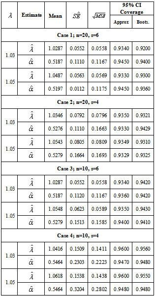
To evaluate and compare the performance of the methods of inference described in present model, first generate a random sample where . The values of the parameters , and are chosen. The values of are chosen close to since the decreasing trend of lifetimes in practice is usually not pronounced. The number of stress levels are chosen to be the number of test products at each stress level is. The estimators and the corresponding summary statistics are obtained by our proposed model and the Newton iteration method. 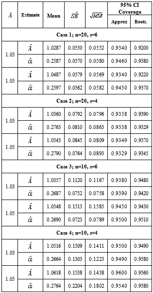For a given sample with different choices of and , the average of the ML estimations (mean), the sample standard deviation of the estimates the average of asymptotic standard error , the square root of mean squared error and the coverage rate of the 95% confidence interval for and are obtained. The CIs are obtained by two methods: the asymptotic distribution and the parametric bootstrap. 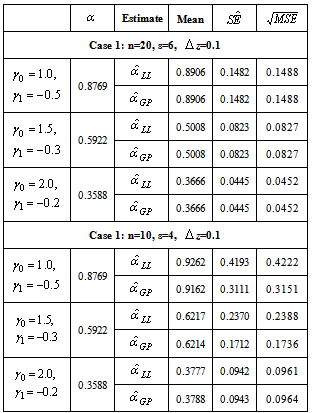Table-1 and 2 summarize the results of the estimates for and. The numerical results presented in Table-1 and 2 are based on 750 simulations and 750 bootstrap replications.

Now to compare the estimation performances geometric process and log linear model, choose the first stress level to be and the difference between each ascending stress level to be . Consequently, the normal stress level would be . Three pairs of parameters are chosen andon the basis of the Xiong’s[18] simulation study. With the prefixed parameters and, the distribution parameter could be easily obtained by . For known values of together with and , the estimates of , the asymptotic standard error of , and the square root of mean squared error , are obtained by both geometric process and log linear model. The numerical results are based on 750 replications and presented in Table-3.

Table 1. Parameter Estimation for the complete simulated sample with α=0.5, β=1

Table 2. Patameter Estimation for the completesimulated sample with α=0.25, β=1

Table 3. Comparison between the GP and the Log Linear(LL) Model

7. Conclusions

From results in Table 1 and 2, it is observed that and estimate the true parameters and quite well respectively with relatively small mean squared errors. The estimated standard error also approximates well the sample standard deviation of the 750 estimates. For a fixed and we compare their estimates across the four different cases and find that as and decreases, the mean squared errors of and get larger. This may be because that a larger sample size results in a better large sample approximation for the distribution of and, so the inference for the parameters is more precise. It is also noticed that the coverage probabilities of the asymptotic confidence interval are close to the nominal level and do not change much across the four cases. The parametric bootstrap confidence intervals have similar coverage rates as the asymptotic CIs.

The results in Table 3 indicate that most of the estimates from the geometric process model match the values obtained by the log linear model. It is seen that when the sample size and number of stress levels are relatively small, some of the estimates obtained by geometric process model have a smaller mean square error than that obtained by the log linear model. It is also noted that some estimates obtained by geometric process have a greater mean square error, but those differences are relatively very slight.

In summary, the proposed geometric process model has a promising potential in the analysis of accelerated life testing when the stress increases arithmetically. It depicts the decreasing trend of lifetimes over increasing stress levels in an intuitive way and provides a simple form to derive the estimates of parameters at normal stress level. Therefore, it is reasonable to say that the proposed model works well.