-
Paper Information
- Previous Paper
- Paper Submission
-
Journal Information
- About This Journal
- Editorial Board
- Current Issue
- Archive
- Author Guidelines
- Contact Us
International Journal of Statistics and Applications
2012; 2(4): 40-46
doi: 10.5923/j.statistics.20120204.03
Statistical Modeling for Wheat (Triticum Aestivum) Crop Production
 Abstract
 Reference
 Full-Text PDF
 Full-Text HTML
Rajarathinam Arunachalam , Vinoth Balakrishnan
Manonmaniam Sundaranar University, Tirunelveli , 627 012, Tamil Nadu, India
Correspondence to: Rajarathinam Arunachalam , Manonmaniam Sundaranar University, Tirunelveli , 627 012, Tamil Nadu, India.
| Email: |  |
Copyright © 2012 Scientific & Academic Publishing. All Rights Reserved.
The present investigation was carried out to study the trends in area, production and productivity of wheat crop grown during the period 1950-1951 to 2009-2010 in India. Different non-linear models were employed to study the trends in area, production and productivity. When none of the non-linear models were found suitable to fit the trends nonparametric regression model was employed. None of the non-linear model was found suitable to fit the trends in area data. The Sinusoidal model was found suitable to fit the trends in production as well as productivity of wheat crop grown in India. The results indicated that area, production and productivity of wheat crop grown in India, had been shown in the increasing trend. The area of cultivation had played a major role in increasing the trend in production.
Keywords: Adjusted R2, Durbin-Watson Statistic, Root Mean Square Error, Mean Absolute Error, Kernel Density, Bandwidth, Cross Validation
Article Outline
1. Introduction
- Wheat is a cereal grain which originated in from the Levant region of the North east but is now cultivated globally. In 2007 world production of wheat was 607 Million Tons, making it the third most produced cereal crop after maize and rice. Wheat’s particular characteristic i.e. it’s adaptability has favoured its growth worldwide. Wheat is adapted to a wide variety of climatic conditions. It is grown where annual temperatures of 4.9 to 27.8℃ prevail [3].When we look at the major producers Globally, China emerges as the leading producer of wheat followed by India at second place, and USA ranks third amongst the top producers globally. On an average, China produces 108,712 TMT of wheat annually, making it the worlds largest producer of wheat but it is not enough to feed its 1.2 Billion population thus it is forced to import 4,247 TMT of wheat and it also exports a very little amount to the neighbouring Asian countries about 657 TMT annually. India is second largest producer of wheat in the world, averaging an annual production of 65,856 TMT. Although it is less when compared to china but India imports less comparatively, also India has a population almost comparable with that of China. India imports 990 TMT of wheat, and, for various reasons, exports an average of 767 TMT of wheat annually[2]. The country's wheat production is estimated to achieve an all-time high of 81.47 million tons and the overall food grain output is projected to rise by over 6% to 232.07 million tons in 2010-2011 crop year. The bumper harvest is expected to contribute significantly to the economic growth. The government had projected 8.6% expansion in the economy, aided by an impressive 5.4% rise in agriculture and allied activities [3, 4].Thus this shows the significance of wheat in India and therefore the statistical information on the area, production and productivity of the crop emerges as a subject of great importance. Measurement of growth rate in agricultural productions looks apparently simple, but it is not free from complications. Thus the experimental analysis of different statistical model like the parametric (Linear or Non-linear models) by assuming the linear or exponential functional forms and nonparametric models is mandatory to get the statistical estimation of the productivity of the crop and its future predictions.A number of research workers [8, 9, 13, 14, 15, 18, 19, 21, 22, 28 and 29] have used parametric models to estimate growth rates. There are the drawbacks of these models i.e. the data may not be following these linear or exponential models or may require fitting of higher degree polynomials or non linear models. Further, these models lack the economic considerations i.e. normality and randomness of residuals [26]. Thus recourse to the nonparametric regression approach is taken which is based on fewer assumptions [11].The same is done in this paper, non-linear and nonparametric models are applied, to study the trends in production of the wheat crop and developing a best possible statistical model for analyzing the area, production and productivity of the wheat crop data.
2. Materials and Methods
- The time-series data on area, production and productivity for the period 1950-1951 to 2009-2010 were collected through the web site www.agricoop.nic.in. The data were analyzed using the non-linear as well as the nonparametric regression models and the conclusion is given based on the best model to study the trends and growth rate of wheat crop production in India.
2.1. Non-Linear Models
- In parametric model, different non-linear models[5, 10, 17, 25 and 27] given in Table 1 were employed. Among the non-linear models, the model having highest adjusted R2 with significant F value was selected, so that it satisfied test for goodness of fit[17]. Normality of residuals was examined by using Shaprio-Wilks test[1]. Further more, while dealing with time-series data it may be possible that successive observations may be auto-correlated among themselves[30]. To overcome all these problems, performing residual analysis was being carried out. Randomness assumption of the residuals required to be tested before taking any final decision about the adequacy of the model developed. To carry out the above analysis “Run test” procedure developed in the literature [25] was used. Further, to test the presence or absence of auto-correlation in the data set Durbin-Watson test procedure[16] was utilized In case of more than one model being the good fit for the data, the best model was selected based on lower values of Root Mean Square Error (RMSE) and Mean Absolute Error (MAE) values.Levenberg-Marquardt algorithm[25] which is widely used was utilized for fitting Logistic, Gompertz Relation, Sinusoidal and Rational Function. Different sets of initial parameter values were tried so as to ensure global convergence. The iterative procedure was stopped whenever the successive iterations parameter estimates values were negligibly low. The standard SPSS Ver. 16.0 package was used to fit all the models given in Table 1.
2.2. Nonparametric Regression Model[11, 12]
- The nonparametric regression model with the additive error is of the form
 where Yi is the observation (area, production and productivity) of the ith time point, m is the trend function, which is assumed to be smooth, and
  is random error with mean zero and finite variance
 . The kernel weighted linear regression smoother is used to estimate the trend function. The value of the local linear regression smoother at time x is the solution of a0 to the following weighted least squares problem:
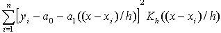 where K is a bounded symmetric kernel density function and h is the bandwidth. Let
  and
and  be the solutions to the weighted least squares problem. The estimate of the trend function m(t) is given by
 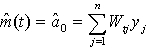 where
where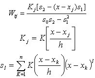 The optimum bandwidth h can be obtained by the method of cross-validation. The slope m|(x) of m(x) can be considered as the simple linear growth rate at the time point x. The estimate of m|(x) is given by
 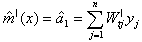 where
where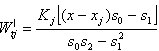 .
.3. Results and Discussion
- Different non-linear and nonparametric regression models were employed to study the trends in the area, production and productivity data of the wheat crop. The findings are discussed in sequence, as follows.
3.1. Trends in Area
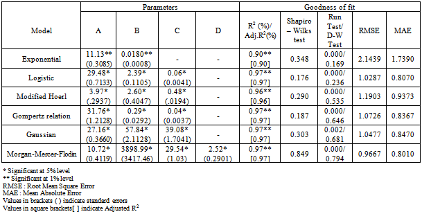
- The data presented in Table 2. for the area under the wheat crop revealed that among the non-linear models fitted to the area under the wheat crop, the maximum adjusted R2 of 97 per cent was observed in case of Morgan-Mercer-Flodin (MMF) model with comparatively lower values of RMSE (0.9667) and MAE (0.8010) in comparison to that of other non-linear models. The Shapiro-Wilks test (test for normality) was found to be non-significant indicating that the residuals due to this model were found to be normally distributed. However the run test (test for randomness) value was significant indicating that the residuals were correlated.Y=(10.72*3898.99+29.54*X^2.52)/(3898.99+X^2.52)(R2=97%)Since none of the non-linear models was found suitable to fit the trends in area under the wheat crop, the nonparametric regression model was employed to fit the trends in area data. The optimum bandwidth was computed as 0.50 using the cross-validation method. Nonparametric estimates of underlying growth function were computed at each time point. Residual analysis showed that the assumptions of independence of errors were not violated at 5%level of significance. The RMSE and MAE values were found to be 0.5069 and 0.4107 respectively. These values were found to be much lower than those obtained through the parametric models, indicating thereby the superiority of this approach over the parametric approach. Hence the nonparametric regression model was selected to fit the trends in area under the wheat crop. The graph of the fitted trend for area under the wheat crop using the nonparametric regression is depicted in the Fig 1. Similar trends were observed for Gujarat wheat production [7].Nonparametric regression model was used [24] to fit the trends in tobacco crop grown in Anand district of middle Gujarat in India for the period 1949-1950 to 2007-2008.
|
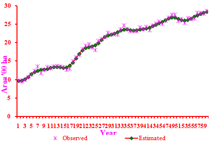 | Figure 1. Trends in area of wheat crop based on nonparametric regression |
3.2. Trends in Production
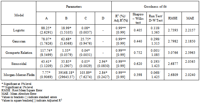
- In case of the production of wheat crop, the Sinusoidal model had maximum adjusted R2 of 99 % with the comparatively lower values of RMSE (2.6877) and MAE (2.0565) among the parametric models fitted to the production of the wheat crop. Moreover, the run tests as well as the Shapiro-Wilks test values were non-significant indicating that the residuals due to this model were independently normally distributed. All the estimated parameter values were in the 95 % confidence interval indicating that the parameter values were significant (Table 3).Y = 43.41 + 35.85 * COS(0.0513*X+2.94) (R2=99 %)The graph of the fitted trend for the production of wheat crop using the Sinusoidal Model is depicted in the Fig 2.
|
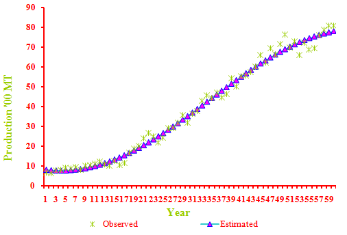 | Figure 2. Trends in production of wheat crop based on Sinusoidal model |
3.3. Trends in Productivity
- The data presented in Table 4 for productivity of wheat crop revealed that among the non-linear models fitted, the maximum adjusted R2 of 99 per cent was observed in the case of Sinusoidal model with the comparatively lower values of RMSE (85.5915) and MAE (69.5027). All the estimated values of the parameters in the model were found to be within the 95% confidence interval indicating that the parameters were significant at 5% level of significance. The Shapiro-Wilks test (test for normality) and run test (test for randomness) values were found to be non-significant indicating that the residuals fulfilled model selection criteria. Among the non-linear models, the sinusoidal model was found suitable to fit the trends in productivity of wheat crop.Y = 1756.28+1043.13*Cos(0.06*X+2.92) ( R2 = 99* %)The graph of the fitted trend in productivity of wheat crop using the Sinusoidal Model is depicted in the Fig 3.
3.4. Discussions in area, production and productivity of wheat Crop
- In the present study exponential model was not found suitable as the best fitted model because of lack of assumptions of residuals, though some earlier reports [6,31] found exponential model as suitable. Hence the nonparametric regression model was selected as the best fitted trend function for the area under the wheat crop. The Sinusoidal model was found suitable to fit the trends in production as well as productivity of wheat crop grown in India.
|
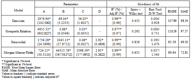
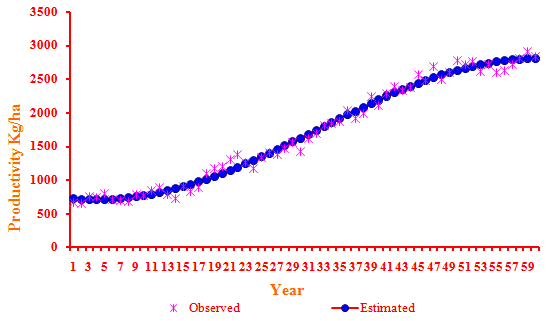 | Figure 3. Trends in productivity of wheat crop based on Sinusoidal model |
4. Conclusions
- From the above discussion on the analysis of area, production and productivity of wheat crop data based on different non-linear as well as nonparametric regression models, it can be finally concluded that, the parametric models (non-linear) are based on many assumptions and they go on the current condition of the crop and other parameters at a particular instant of time. It is not dynamic enough to be considered as a suitable method for the calculation or the estimation of the growth rate of the wheat crop. Nonparametric model was found to be a suitable measure to estimate the growth rates of the wheat production data grown in India because it is based on fewer assumptions i.e. this model can be used as a most suitable one as it is dynamic and versatile enough to be considered for the statistical interpretation for the growth and trends for the wheat crop for the years to come.The Sinusoidal model was found suitable to fit the trends in production as well as productivity of wheat crop grown in India. The area, production and productivity of wheat crop grown in India, had been shown in the increasing trend. The area of cultivation had played a major role in increasing the trend in production.
ACKNOWLEDGEMENTS
- The financial assistance received by the second author in the form of JRF from University Grant Commission (UGC) of the Indian Government is highly acknowledged.
References
| [1] | Agostid’no, R.B., Stephens, M.A., (1986). “Goodness of fit technologies”, Marcel Dekker, New York . |
| [2] | Anonymous Courtesy: USDA Economic and Statistics System,spectrumcommodities.com/education/commodity/statistics/wheat |
| [3] | Anonymous,(2011(a)).(dnaindia.com/india/report_wheat-production-expected-to-reach-all-time-high-in-2011_1505146) |
| [4] | Anonymous,(2011(b)).(rediff.com/business/report/india-gains-as-wheat-production-dips-in-us-china/20110421.htm) |
| [5] | Bard, Y., (1974). “Nonlinear Parametric Estimation”, Academic Press, New York. |
| [6] | Bera, M.K., Chakravarty, K., Shahjahan Md., and Nandi, S., (2002). “Area, production and productivity of rice in major rice growing districts of West Bengal during nineteen eighties”. Economics Affairs, 47(2):108-114. |
| [7] | Bhagyashree, S.D., (2009). “Application of parametric and nonparametric regression models for area, production and productivity trends of major crops Gujarat”. M.Sc. Thesis, Submitted to Anand Agricultural University, Anand, Gujarat. |
| [8] | Borthakur, S., Bhattacharya, B.K., (1998). “Trend analysis of area, production and productivity of potato in Assam”: 1951-1993. Economic Affairs, 43: 221-226. |
| [9] | Dey, A.K., (1975). “Rates of growth of agriculture and industry”. Econ. Political Weekly, 10: A26-A30. |
| [10] | Draper, N.R., Smith, H., (1998). “Applied Regression Analysis”. 3rd Edn., John Wiley and Sons, New York, USA |
| [11] | Hardle, W., (1990). “Applied Nonparametric Regression”. 1st Edn., Cambridge University Press, New York, USA. |
| [12] | Jose, C.T., Ismail, B., and Jayasekhar S., (2008). “Trend, Growth rate, and Change point Analysis – A Data Driven Approach”. Communications in Statistics.- Simulations and Computation, 37: 498-506. |
| [13] | Joshi, P.K., Saxena, R., (2002). “A profile of pulses production in India. Facts, trends and opportunities”. Ind. J. Agric. Econ., 57: 326-339. |
| [14] | Kumar, P., Rosegrant, M.W., (1994). “Productivity and sources of growth for rice in India”. Econ. Political Weekly, 29: 183-188. |
| [15] | Kumar, P., (1997). “Food security: Supply and demand perspective”. Indian Farming,12: 4-9. |
| [16] | Lewis-Beck, S.M., (1993). “Regression Analysis”. Sage Publications, New York. |
| [17] | Montgomery, D.C., Peck, E.A., and Vining, G.G., (2003). “Introduction to Linear Regression Analysis”. John Wiley and Sons, USA. |
| [18] | Narain,P., Pandey, R.K., and Sarup, S., (1982). “Perspective Plan for foodgrains”. Commerce, 145: 184-191. |
| [19] | Panse, V.G., (1964). “Yield trends of rice and wheat in first two five-year plans in India”. J. Ind. Soc. Agric. Statistics, 16: 1-50. |
| [20] | Parmer, R.S., (2010). “Statistical modeling on area, production and productivity of major crops of Middle Gujarat”: A case study. Ph.D. Thesis, Anand Agricultural University, Anand, Gujarat. |
| [21] | Patel, R.H., Patel, G.N., and Patel, J.B., (1986). “Trends and variability in area, Production and productivity of Tobacco in India”. Ind Tobacco J., 18: 3-5. |
| [22] | Patil, B.N., Bhonde, S.R., and Khandikar, D.N., (2009). “Trends in area, Production and productivity of groundnut in Maharashtra". Financing Agric., pp: 36-39. http : // www . afcindia . org.in/march-april2009/35-40.pdf. |
| [23] | Rajarathinam, A and Parmar R.S., 2011.”Application of parametric and nonparametric regression models for area, production and productivity trends of castor (Ricinus communis L.) crop”. Asian Journal of Applied Sciences 4(1): 42-52. |
| [24] | Rajarathinam, A., Parmar, R.S. and Vaishnav, P.R., 2010. “Estimating models for area, production and productivity trends of Tobacco (Nicotiana tabacum) crop for Anand region of Gujarat State, India”. Journal of Applied Sciences 10 (20) : 2419-2425. |
| [25] | Ratkowsky, D.A., (1990).“Handbook of Non-linear Regression Models”. Marcel Dekker, New York. |
| [26] | Sananse, S.L., Maidapwad, S.L., (2009). “On estimation of growth rates using linear models”. Int. J. Agric. Statistics Sci., 5: 463-469. |
| [27] | Seber, G. A. F., Wild, C. J., (1989). “Non-Linear Regression”. John Wiley and Sons, New York |
| [28] | Shah, A.N., Shah, H., and Akmal, N., (2005). “Sunflower area and production variability in Pakistan”: Opportunities and constrains. HELIA., 28: 165-178. |
| [29] | Singh, A., Srivastava, R.S.L., (2003). “Growth and instability of sugarcane production in Uttar Pradesh”: A regional study. Ind. Jn. Agri. Econ., 58: 279-282. |
| [30] | Venugopalan, R., Shamasundaran, K.S., (2003). “Nonlinear Regression : A realistic modeling approach in Horticultural crops research”. Jour.Ind.Soc.Ag.Statistics 56(1):1-6 |
| [31] | Yadav, C.P., Das, L.C., (1990). “Growth trend of rice in Assam”. Economic Affairs, 35,(1) : 15-21. |