1. Introduction

Clustering algorithms have been used in a variety of fields such as chemistry, engineering, medicine, etc.[2]. Given a data set the main goal is to produce a partition with high internal intra-class similarity and high inter-cluster dissimilarity. The majority of papers available in the literature deals with clustering algorithms for numerical data even though categorical data are very common in practical applications. Two well-known non-hierarchical algorithms to cluster categorical data are k-modes[20] and fuzzy k-modes[19], which are direct extensions of the k-means[26] and fuzzy c-means[23], respectively. Some alternative algorithms have been developed to increase the accuracy of k-modes and its efficiency to handle larger data sets. Some of these algorithms are direct variations of the k-modes or fuzzy k-modes (see[4] and[5], for examples). The variations include changing the dissimilarity measure used to compare the objects to the cluster centroids or the cluster centroids themselves by adding more information from the data set in their definition besides of using the hard mode. The k-representatives[12] and the k-populations ([9],[1]) are examples of fuzzy k-modes variations. Among the algorithms based on different concepts to cluster data we find the hierarchical method ROCK[17], which uses thenumber of links between objects to identify which are neighbors and belong to the same cluster; the entropy-based algorithms LIMBO[13] and COOLCAT[14]; STIRR[16] based on nonlinear dynamical systems from multiple instances of weighted hypergraphs; GoM a parametric procedure based on the assumption that the data follow a multivariate multinomial distribution ([3],[25])); MADE[3] which uses concepts of the rough set theory to handle uncertainty of the partition; CACTUS[18] based on the idea of co-occurrence between attributes and pairs defining a cluster in terms of a cluster´s 2D projections; the subspace algorithms SUBCAD[11] and CLICK[7] whose main goal is to locate clusters in different subspaces of the data set with the purpose of overcome the difficulties found in clustering high-dimensional data; many other algorithms can be found. Hierarchical agglomerative clustering algorithms such as Single, Complete or Average linkage[15] have also been used to cluster categorical data although non-hierarchical methods are more efficient to handle larger data sets.

Many studies are found in the literature comparing the efficiency of clustering algorithms for categorical data. However, most of them uses benchmark data as references to evaluate the performance of the algorithms. The accuracy of the algorithm is then achieved by comparing the reference data with the partition produced by theapplication of the algorithm to the data. By doing so, the performance of the algorithm is dependent upon the relationship between the reference (previous) partition with the categorical variables used to cluster the data. By using this approach, a reasonable clustering algorithm may be considered of poor performance if the previous partition was created by using criteria with no relationship with the observed categorical variables. On the other hand, any algorithm which works well for these particular benchmark data may be considered very accurate. Therefore, simulation studies are also necessary.

In Kim et al.[9] the k-populations algorithm was proposed as an extension of fuzzy k-modes. In this method a degree of importance of each category of the variables used to group the data was incorporated in the definition of the clusters centroids. The effectiveness of the algorithm was tested using four benchmark data sets[22] having different composition with respect to the number of clusters (k), number of variables (m) and number of data points (n): the soybean, the zoo database, the credit approval and the hepatitis data. The results showed that k-populations algorithm was more accurated than k-modes, fuzzy k-modes and the hierarchical algorithm using Gower’s similarity coefficient[21]. Although the superiority of k-populations was outstanding, further research is necessary to confirm its accuracy since the algorithm was tested only in four particular data sets. Taking that into consideration, the purpose of this paper is to evaluate the k-populations performance by using Monte Carlo simulation as well as to compare it to four clustering algorithms for categorical data: average linkage, ROCK, k-modes and fuzzy k-modes. The average linkage is a hierarchical procedure available in the majority of the statistical software and it has been proved to be a reasonable method to cluster numerical data (see[8] and[24]). ROCK is very appealing and its good performance has also been demonstrated in studies by using benchmark data sets. However, as far as we know, no paper has been published in the literature comparing these 5 algorithms using reference data sets or Monte Carlo simulation.

2. Clustering Algorithms for Categorical Data

2.1. k-Modes

The k-modes algorithm proposed by Huang[20] to cluster data on categorical variables is an extension of k-means[23]. It uses a dissimilarity coefficient to measure the proximity of the clusters, modes instead of means, and a frequency-based method to update the modes in each step. Let be a sample observation described by categorical variables being the domain of each denoted by, and let be the observed value of for . The objective function of k-modes which has to be minimized, is given by:

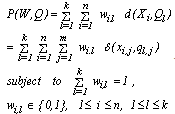(1)

where is the vector mode of the cluster ,,; m is the number of categorical variables and is the dissimilarity measure defined as

(2)

The basic steps of the algorithm are as follows: (i) k initial modes are selected and each object is compared to them by means of (2) being allocated in the nearest group; (ii) after the allocation of all elements, the k modes are updated and the allocation step is repeated again. The algorithm stops when there is no reallocation among the objects into clusters. As pointed out by Huang[17], k-modes may terminate at a local optimum rather than a global optimum solution and the final partition depends on the initial modes and the ordering of the objects of the data set.

2.2. Fuzzy k-Modes

The fuzzy k-modes algorithm was proposed by Huang and Ng[19] as an extension of the k-modes and it is based on the fuzzy c-means algorithm used to cluster numerical data[23]. Two new parameters are added in this method: the degree of membership (w) of the observations to each cluster, , and the fuzzy parameter denoted by . The membership degrees are estimated in the execution of the algorithm; the fuzzy parameter is fixed in advance and controls the degree of overlapping expected among clusters. In the literature is very common to set . The degree of chaos in the final partition increases as goes to infinity.

The objective function of the fuzzy k-modes, which has to be minimized to produce the best partition, is given by

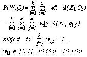(3)

where and are defined as in section 2.1.

According to Huang and Ng[16] the function (3) is minimized if and only if and such that

(4)

where is given as (5). As in k-modes the vector modes may not be unique.

(5)

The basic steps of the fuzzy k-modes, for k and fixed, are as follows: (i) for each object i and each cluster l, the degree of membership is selected and normalized. It can be randomly chosen from the uniform distribution defined in the[0,1] interval for example; (ii) k initial modes are selected by using equation (4); (iii) all objects are compared to the modes using a dissimilarity measure and allocated to the nearest group; (iv) the weights are recalculated according to equation (5) and the modes are updated; (v) the steps (iii) and (iv) are repeated till there is no change in the clusters modes.

Fuzzy k-modes has been proved to be an efficientclusteralgorithm with the advantage of pointing out the data points which share some similarity with different clusters of the partition and therefore could be misclassified by k-modes-type of algorithms.

2.3. k-Populations

A modification of fuzzy clustering algorithm, called k-populations, was proposed by Kim et. al.[9]. In this new procedure the mode of cluster l, called the population of the lth cluster centroid, is denoted by and it is defined as , where

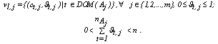Therefore, the composition of the fuzzy centroids is determined by the categories and by the contribution degree of these categories to the specific cluster, , which is defined as

(6)

where

and denotes the category t of variable . Briefly speaking, for each category t of the variable , describes the category distribution of the attribute for data belonging to the lth cluster. The normalizing factor , is the length of the vector , where is the degree of membership as defined in section 2.2. According to Kim et. al.[9] the introduction of the minimizes the imprecision in the representation of cluster centroids and improve the efficiency of the fuzzy clustering algorithm in finding the optimal partition rather than a local optimal.

As an illustration suppose there is only one categorical variable with two possible categoriesand that for a given cluster l , there are 3 observations Therefore, .

Let , , and Then, since for the category t=1 of, ,and . Similarly, it is found and the fuzzy centroid is given by .

In k-populations the dissimilarity measure used to compare any observation to any fuzzy centroid is given by

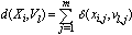(7)

where

being a the normalization factor which corresponds to the length of the vector.

For k and fixed, the basic steps of the k-populations algorithm are given as follows: (i) choose k initial seeds (fuzzy centroids) and the degree of contribution at random; (ii) obtain the proximity matrix between the observations and the fuzzy centroids according to equation (7); (iii) estimate the degree of membership according to the equation (5) and update the fuzzy centroids according to equation (6); (iv) repeat steps (ii)-(iii) until there is no reallocation of objects into clusters.

2.4. The Average Linkage

The Average linkage is a well-known algorithm used to cluster categorical and numerical data[15]. It starts with each object as its own cluster (step 1); the similarity between clusters are calculated and the two most similar are merged (step 2); this last step is repeated over and over again till the desirable number of clusters k is achieved.

Let and be two clusters with sizes and , respectively. In the Average linkage the dissimilarity measure between these two clusters is defined as:

(8)

where is any dissimilarity measure used to compare the and elements. Average linkage does not depend on the notion of initial seeds and therefore, its final partition is not affected by the ordering of the objects in the data set. However, computationally speaking it is less efficient than non-hierarchical algorithms for large data sets.

2.5. ROCK (RObust Clustering using linKs)

Different than other cluster algorithms ROCK, proposed by Guha et. al.[17] is based on the notion of links instead of distance or dissimilarity to cluster objects. The number of links between two objects represents the number of neighbors they have in common in the dataset. Let s(.) be a similarity measure. Two observations and are considered neighbors if , where is a pre-specified threshold parameter which controls the amount of similarity required for two observations to be considered neighbors. The is the number of neighbors the two observations have in common; the higher is its value the more probable is that and belong to the same group. The main goal is to maximize the sum of links between the observations which belong to the same group and to minimize the sum of links between observations which belong to distinct groups.

In practice the implementation of ROCK is as follows: after an initial computation of the number of links between the data objects, the algorithm starts with each cluster being a single object and keeps merging clusters till the specified number of clusters is achieved or no links remain between the clusters. In each step of the algorithm the two clusters which maximizes the goodness measure given in (9) are merged, where and are the clusters being compared and is given by (10). The quantity in the denominator of (9) is approximately the expected number of cross links between the pair of clusters and is a pre-specified function. According to Guha et. al.[17] empirical work had been shown that the function works well in practical situations. Under this function when the expected number of links in cluster is approximately equal to , i.e., each sample point is a neighbor of itself; when the expected number of links in cluster is approximately equal to, which corresponds to the situation where all the observations in are neighbors of each other.

(9)

(10)

In Guha et. al.[17] ROCK was implemented using the Jaccard similarity measure. However, an improvement of the computational efficiency of the algorithm is achieved when the weighted similarity measure given in (11) is applied (see[10]). According to (11), for each attribute it is associated a weight proportional to its number of categories. By doing so a pair of observations differing in only one variable whose domain has two categories will have a smaller similarity value than a pair also differing in only one variable, but whose domain has a larger number of categories.

(11)

3. Monte Carlo Simulation

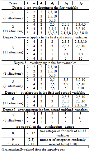
A total of 64 population structures of clusters were simulated considering different degrees of overlapping among clusters, different number of clusters and categorical variables (k=2,3,5; m=2,4,15) and different number of categories (t=2,3,5,10). Each generated cluster had 50 observations and the population structures of clusters were simulated to possess features of internal cohesion and external isolation. Additionally, one population structure was simulated without pre-setting the values of k,m,t in advance, but by selecting them randomly from the sets: {2,…,8}, {2,…,15} and {2,…,10}, respectively.

The main objective of the simulation study was to evaluate the changes in the performance of the clustering algorithms from more stable situations (smaller degree of overlapping, number of clusters, variables and categories), to more complex situations (higher degree of overlapping, number of clusters, variables and categories).

3.1. Data Generation

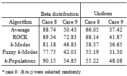
Table 1 presents the simulated population structures grouped by cases. Each case represents a different situation in terms of overlapping. Clusters without overlapping were generated in cases 1 and 2 (degree 1: non-overlapping in the first variable) and case 3 (degree 2: non-overlapping in the first and second variables). Overlapping clusters were generated in cases 4 and 5 (degree 3: overlapping in the first variable), case 6 (degree 4: overlapping in the first and second variables) and case 7 (degree 5: overlapping in the first three variables). The non-overlapping clusters were built as follows: all observations of the same group had the same category on the first variable (cases 1 and 2) or for the first and the second variables (case 3). The categories of the remaining variables (for m>2) were generated randomly according to the Beta and the Uniform distributions. As an illustration consider case 1, k=2, m=2 and t=2, and suppose that {a,b} are the categories of the first variable. The two clusters were built as follows: for the first variable the category {a} was allocated to all the observations of the first cluster and the category {b} for all observations of the second cluster. For each object the category of the second variable was generated randomly for both clusters. Now consider the case 3, k=5,m=4, the first variable with categories {a,b,c,d,e} and the second variable with categories {f,g,h,i,j}. Then for the first cluster, the categories {a} and {f} were allocated to all objects for the first and second variables, respectively; for the second cluster the categories {b} and {g} were allocated to all objects; and following this procedure for the cluster five the categories {e} and {j}, respectively, were allocated to all objects. For the other two remaining categorical variables the observations were generated randomly for each cluster.

The overlapping, (cases 4-7), was performed in such way that all the categories of the variables used to build the overlapping had proportionally the same frequency for each cluster. For example, suppose k=2, m=2, each variable with 2 categories (case 4). Then, the simulation procedure assured that the first category of variable 1 would appear in half of the observations of cluster 1 and the second category in the other half. The observations of the second variable were randomly generated. The same procedure was used for cluster 2. Now suppose k=5, m=4, each variable with 5 categories (case 7). Then for each cluster, for the first, second and third categorical variables, the simulation procedure assured that the frequency of each category would be equal to 20% from all observations from the respective cluster. The observations for the other two remaining categorical variables were generated at random. The proportionality was preserved even in situations where the variables used to build the overlapping had different number of categories.

In all situations the generation of the observations for the remaining variables not used in the overlapping procedure, was performed according to the Beta and the Uniform distributions as follows. For each cluster, and each category of the variable j=1,2,…,m, a random number was selected from the Uniform distribution defined on the[0,1] interval and the Beta distribution with parameters and The vector of the generated numbers from each distribution was normalized to describe the probability of observing each category of . Data for all categories of were then generated randomly according to the correspondent normalized probability vector. The Uniform model represents the situation where all categories of had approximately the same chance of being observed. The Beta distribution was chosen to describe situations where some categories of would have higher chance to appear in the sample than others, which is common in practical applications. As an illustration, Figure 1 presents the results of 4 samples of size 50 of a variable with 3 categories, generated by the described procedure. As it can be seen the Uniform distribution tends to generate classes with similar frequencies different than the Beta distribution which tends to produce classes with larger frequencies than others.

Due to the fact that the values for the variables not used to build the overlapping were generated randomly, there is a chance of possible overlapping among the clusters generated in cases 1-3.

In the case 8 (k=2,m=2,t=15) there was no control of the overlapping degree among clusters since for each cluster, the observations were randomly selected from the Uniform and Beta distributions. Finally, the case 9 represents the situation where there was no control in the simulation for the number of clusters, variables and categories as well as for the degree of overlapping. For this case, the number of clusters was randomly selected from the set {2,3,…,8}, the number of variables from the set {2,3,…,15} and the number of categories from the set {2,3,…,10}. The observations for each cluster were generated from the Beta and the Uniform distributions, as previously described.

From each cluster structure of Table 1 a total of 1000 runs were simulated. The elements of each run were clustered into k groups by using all five clustering algorithms presented in section 2. The resulted partitions were then compared with the true simulated population structure and the performance of the algorithm was evaluated by the average percentage of correct classification taken over 1000 runs (called recovery rate).

Table 1. Simulated structures: number of clusters, variables, categories and degree of overlapping

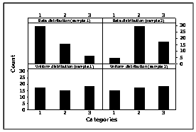Figure 1. An illustration of samples from Beta and Uniform distributions. Simulated data – sample size 50

For each run of the Monte Carlo simulation the criterion used to interrupt the execution of the average linkage andand ROCK algorithms was the pre-specification of the number of clusters. For each simulated data the initial seeds needed for the execution of k-modes, fuzzy k-modes and k-populations algorithms were randomly chosen from the simulated data by using sampling without replacement. The fuzzy parameter was set as 2 and in the final partition each object was assigned to the cluster whose estimate was the largest. The dissimilarity measure given in (11) was used in all algorithms.

4. Results and Discussion

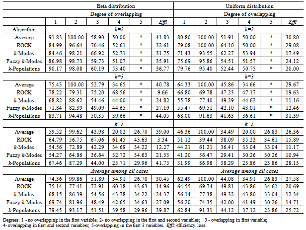
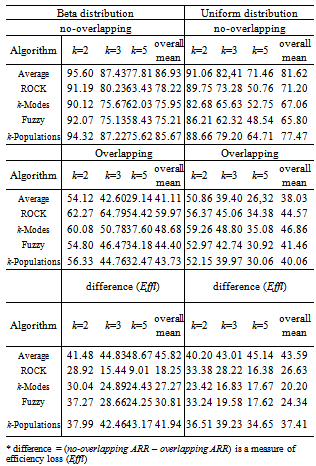
To evaluate the performance of the algorithms the average of recovery rates (ARR) was calculated considering all factors involved in the simulation procedure: degree of cluster overlapping, number of clusters (k) and variables (m). The results are shown in Table 2 for each algorithm according to the degree of overlapping and the distribution used to generate the data. A weighted overall performance mean is also presented and it was calculated taking into account the fact that the number of simulated models were not the same for each combination of k, m and degree of overlapping. It can be seen that for each clustering algorithm and each k, the larger is the degree of overlapping the smaller is the ARR values, as expected. The same is true when the number of clusters increased. However, the performance loss due to the increase of overlapping degree from 1 to 4 does not necessarily increase with the number of clusters neither is similar for all algorithms. In all situations the average recovery rates were larger for data generated from the Beta distribution. The best results were achieved for k=2 and degrees 1 and 2 of overlapping (for Beta data; ; for Uniform data). When k=2 and the degree of overlapping increased to 3 and 4, the ARR values dropped down ranging from 51.07 to 76.46% (Beta data) and 50 to 64.1% (Uniform data). When k increased to 3 the ARR values decreased ranging from 55.47 to 100% for degrees 1 and 2 of overlapping and from 34.65 to 75.2% for degrees 3 and 4, taking into account data from both distributions. The larger impact took place when k=5 since the majority of the ARR values belongs to theinterval[20,65%] except for average linkage and k-populations which presented ARR values between 70 to 80% for non-overlapping data. Considering all the situations, average linkage and k-populations were the most affected by overlapping as it can be seen by the efficiency loss values (Effl) which is defined as the difference between the ARR values from degrees 1 and 4 of overlapping (see Table 2). On the contrary, ROCK was the less affected and the only method resulting ARR values larger than 50% in all situations for Beta data except for the degree 5 of overlapping, although being also the best in this situation. For Uniform data k-modes was the less affected by overlapping.

Table 2. Average recovery rates for all algorithms according to the overlapping degree (m=4)

The 63 simulated population structures (cases 1 to 7) were grouped into the “no-overlapping cases” (i.e. degrees 1 and 2 of overlapping) and “overlapping cases” (degrees 3 and 4 of overlapping) and the average recovery rates were taken over all the simulated structures belonging to each respective group. The main results are shown in Tables 3 and 5 according to the number of clusters and variables for both types of generated data. The overall averages taken among all 63 simulated population structures are also shown. Table 4 presents the difference between the average recovery rates for all clustering algorithms calculated using the overall means shown in Table 3. From these results (Tables 3 and 4), it is seen that in average, for the “no-overlapping” group, the average linkage and k-populations were the best algorithms (overall means over 85%) compared to ROCK, k-modes and fuzzy k-modes (overall means between 75 and 78%). It is important to point out that the best average recovery rates were found for k=2 (overall means over 90%). For the “overlapping group” and data from a Beta distribution, ROCK was the best with ARR values larger than any other clustering method (overall mean 59.97%). The average linkage was the less accurate (overall means of 41.11% and 38.03% for Beta and Uniform data, respectively) followed by k-populations (overall means of 43.73% and 40.06% for Beta and Uniform data, respectively). Under overlapping the difference between the average recovery rates were smaller for data coming from the Uniform distribution being k-modes and ROCK the best algorithms although the overall means were very small (46.86% for k-modes and 44.57% for ROCK).

The results from Table 5 show that the ARR values were similar for m=2 and m=4 categorical variables. Comparing the ARR values from Tables 3 and 5 it is easily seen that the increase of the number of categorical variables had less impact in the accuracy of the algorithm than the increase of the number of clusters.

The efficiency loss measured by the difference between the “no-overlapping” and “overlapping” average recovery rates (see Tables 3 and 5) corroborate to the fact that average linkage and k-populations were the most affected by overlapping (average efficiency loss equal 45.82 and 41.94%, respectively) as long as ROCK (for Beta data) and k-modes (for Uniform data) were the less affected (average efficiency loss equal 18.25 and 20.20%, respectively).

Table 6 presents the results for cases 8 and 9, the two situations simulated with no control on the overlapping degree. For case 8 the average recovery rates were higher than 77% for data from the Beta distribution and between 55.19 to 68,14% for data from the Uniform distribution, results very reasonable for a situation whose number of clusters and categories were small (2) and the number of categorical variables was large (15). On the other hand, when the parameters (k,m,t) were chosen randomly (case 9), the average recovery rates were smaller (under 54.85%), specially for data from the Uniform distribution. The only exception was ROCK with an average recovery rate equal 72.83% (for Beta data).

5. Final Remarks

Table 3. Average recovery rate for all algorithms according to the overlapping degree

Table 4. Difference between the average recovery rates for all clustering algorithms

In this paper the performance of five clustering algorithms for categorical data was evaluated by means of Monte Carlo simulation being Beta and Uniform distributions used to generate the artificial data. The results showed that overlapping is the factor with major impact on the accuracy of all the algorithms. Although the increase in the number of categorical variables affects the performance of the algorithms the impact is smaller than the respective impact due to the increase of the number of clusters. The average recovery rates were larger for data whose categories had difference frequency of occurrence (Beta data) compared to the data whose categories had approximately the same frequency (Uniform data).

Table 5. Average recovery rate according to overlapping degree and number of categorical variable

Table 6. Average recovery rate – no control on the overlapping degree

The superiority of k-populations over to k-modes and fuzzy k-modes presented by Kim et al.[9] was not confirmed by the results shown in this paper. In fact for Beta and Uniform data, the k-populations algorithm presented better accuracy only in cases where there was a small degree of overlapping (degree 1 and 2) having performance similar to the average linkage algorithm which was the best for these type of simulated situations. However, similar to the average linkage, the performance of k-populations decreased more than 40% in average when additional overlapping was introduced into the data (degrees 3 and 4 of overlapping) and its accuracy was smaller than ROCK, k-modes and fuzzy k-modes in these cases. Therefore, considering that the main goal is to use a clustering algorithm which in average has better accuracy for no-overlapping as well as for overlapping data, the simulation study has indicated that k-modes, fuzzy k-modes and ROCK should be preferred to k-populations, particularly ROCK which in general, was the algorithm less affected by overlapping and presenting average recovery rates larger or similar than any other algorithm discussed in this paper.

Finally, this paper shows that the evaluation of the accuracy of the clustering algorithms for categorical data should not be restricted to the studies which only use benchmark data to estimate their performance. It is also important to conduct studies using Monte Carlo simulation since by knowing in advance the characteristics of the simulated dataset it is possible to analyse better the impact of factors such as overlapping, number of clusters, categorical variables and categories in the final solution. The drawback of using only real data sets to compare clustering algorithms is the fact that not necessarily the pre-specified partition is consistent with the pattern of the data in terms of the variables used to perform the clustering.

ACKNOWLEDGEMENTS

The authors are very thankful to CNPq and CAPES

Institutions.