M. Salah EL-Sherbeny1, Essam K. AL-Hussaini2
1Department of Mathematics, Faculty of Science, Helwan University, Cairo, P. O. Box 11795, Egypt
2Department of Mathematics, Faculty of Science, Alexandria University, Alexandria, Egypt
Correspondence to: M. Salah EL-Sherbeny, Department of Mathematics, Faculty of Science, Helwan University, Cairo, P. O. Box 11795, Egypt.
| Email: |  |
Copyright © 2012 Scientific & Academic Publishing. All Rights Reserved.
Abstract
In this paper, we investigate the reliability measures: availability  and mean time to system failure
 , for four configurations of series systems with mixed standby components: cold and warm. The time to repair and to failure for each of the operative and warm standby components are assumed to follow the exponential distribution. Comparisons of the computed
 ’s and steady state availabilities
  for the four configurations are obtained for specific values of distribution parameters and cost of the components. The configurations are then ranked based on
  ,
,  and cost/ benefit, where benefit is either
  or
or  . Asymptotic estimation of
  ,
,  and cost/ benefit are computed for the optimal systems.
Keywords:
Availability, Mean Time to System Failure, Asymptotic Estimation, Series System
1. Introduction
Recent technological developments have given rise to the design of many complex systems containing several subsystems to perform different operations in various fields such as defence, industry and systems engineering. Because of the varied nature, these problems have attracted the attention of systems engineers and applied probabilistic. Repairable systems were studied in the past with reference to the evaluation of their performance in terms of reliability and availability. Confidence limits for such measures were studied by[2-6, 10,12]. The cost-benefit analysis of a two-unit cold standby system with two types of repair- minor (regular) and major (expert) are considered by[1,9] studied the optimal system for series systems with mixed standby components.[11] studied the cost benefit analysis of series systems with cold standby components and a repairable service station, when the service times and the failure times of the primary components are assumed exponentially distributed.[8] studied the stochastic analysis of a two-unit cold standby system considering hardware failure, human error failure and preventive maintenance (PM).In section 2, four models are described and assumptions stated. Computations of the MTTF′s are presented in section 3. In section 4, the analyses of steady-state availability for all configurations are introduced. Special cases of the four configurations are compared for different values of the parameters. The cost/benefit ratios are also compared in thissection. The asymptotic estimates of the optimal systems are computed with different measures (cost/benefit) in section 7. Finally, we end up with some concluding remarks.
2. Model Description and Assumptions
We consider a power plant of 10 MW satisfying the following assumptions:1. The system comprises of operative components and mixed standby components “cold and warm”.2. The generators are available in both 10 and 5 MW.3. Standby generators are always necessary in case of failure.4. After a random amount of time, the warm standby component becomes the operative component when the operative component fails; the cold standby component becomes warm standby component, if the standby is available.5. The switchover between the operative and standby components is instantaneous (perfect switch).6. When operative and warm standby components are repaired, they become as good as new.7. Two types of system failure, which are electric and mechanical failures, occur with probabilities  and
and  respectively. 8. Repair and failure rates (warm and operative) are assumed to be exponentially distributed with parameters
 ,
, respectively. 9. Each of the operative components fails independently of the failure of the warm standby component.10. It is assumed those when warm standby component becomes operative, its failure characteristics will be that of operative component and similarly, when a cold standby becomes a warm standby state.The above assumptions are common to all of the following four configurations.
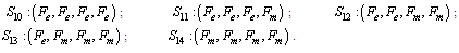
2.1. Configuration Descriptions
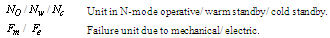
2.1.1. Symbols for the states of all configurations
 2.1.2. Configuration 1Configuration 1 is a serial system of one operative 10 MW component, one warm standby 10 MW component and one cold 10 MW component.Possible states of Configuration 1Up states:
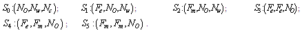 Down states:

2.1.3. Configuration 2
Configuration 2 is a serial system of two operative 5 MW components, one warm standby 5 MW component and one cold 5 MW component.Possible states of Configuration 2Up states: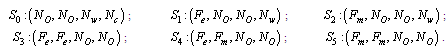 Down states:
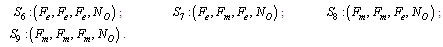
2.1.4. Configuration 3
Configuration 2 is a serial system of one operative 10 MW component, two warm standby 10 MW components and one cold 10 MW component.Possible states of Configuration 3Up states: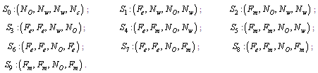 Down states:
2.1.5. Configuration 4
Configuration 4 is a serial system of one operative 10 MW component, one warm standby 10 MW component and two cold 10 MW components.Possible states of Configuration 4Up states: Down states:
2.2. Cost-benefit Factor
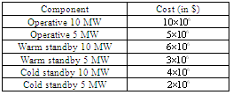
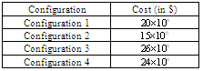
We assume that the size-proportional costs for the primary components and warm standby components are given in Table 1. With this, we calculate the costs for each configuration  shown in Table 2. Let
  be the cost of configuration
  and
and  the benefit of configuration
  , where
  is
is  or
or  .
.Table 1. The size-proportional cost for the operative, warm and cold standby components
 |
| |
|
Table 2. The costs for each configuration

 |
| |
|
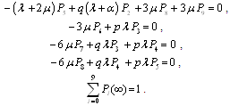
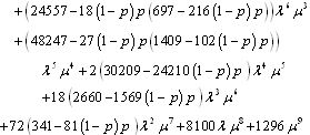
3. Mean Time to System Failure
3.1. Calculations for Configuration 1
Let  be the probability of the states of the configuration at time t
  . If we let
  denote the probability of row vector at time t, then the initial conditions for this problem are
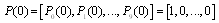 ,Omitting the argument t in
  so that
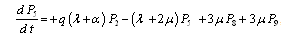
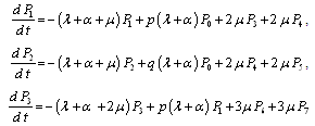
 , we obtain the following differential equations:
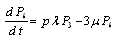
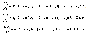
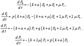 ,
, 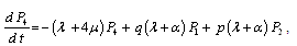 | (1) |
 ,
, ,
, .This can be written in matrix form as
 | (2) |
where is the coefficient matrix for the above equations, 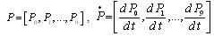 .It is extremely difficult to develop the transient solutions. A simple procedure is provided to develop the explicit expression for the . We delete rows and columns 7,8,9,10 of matrix for the absorbing states to yield a new matrix . The expected times to reach an absorbing state is calculated from
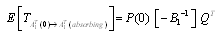 | (3) |
where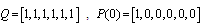 and
and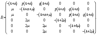 It may be noted that the following relation holds.
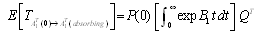 | , (4) |
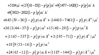
where  .For configuration 1, the explicit expression for the
  is given by
 | (5) |
where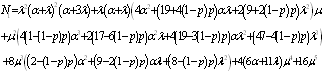 and
and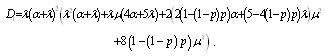
3.2. Calculations for Configuration 2
Application of the above to configuration 2, with  replacing
  in all equations, we obtain
  | (6) |
where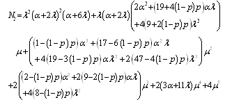 and
and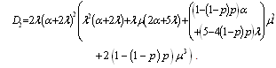 .
.
3.3. Calculations for Configuration 3
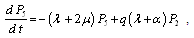
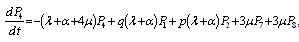
Repeating, as done for configurations 1 and 2, we obtain the following differential equations for configuration 3: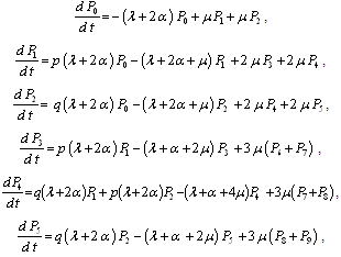 ,
, | (7) |
 ,
, .This can be written in matrix form as
 | (8) |
where is the coefficient matrix for the above equations, 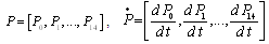 .Rows and columns 10, 11, 12, 13, 14 of matrix
  for the absorbing states are deleted to yield a new matrix
  . The expected times to reach an absorbing state is calculated from
 | (9) |
where  is defined as matrix
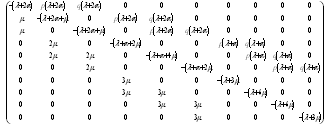 It then follows that
  | (10) |
where
 and
and .
.
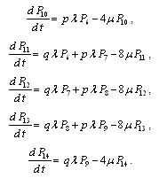
3.4. Calculations for Configuration 4
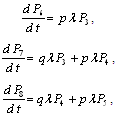
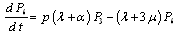
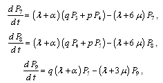
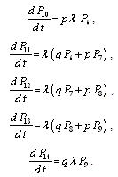
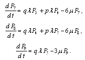
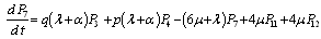
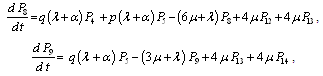
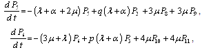
Repeating, as done for configurations 1, 2 and 3, we obtain the following differential equations for configuration 4: 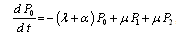 ,
, ,
, ,
, | (11) |
Equations  , …,
, …,  are the same as their corresponding equations in configuration 3.This can be written in matrix form as
 | (12) |
where is the coefficient matrix for the above equations. Rows and columns 10, 11, 12, 13, 14 of matrix for the absorbing states are deleted to yield a new matrix. The expected times to reach an absorbing state is calculated from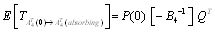 | , (13) |
where  is defined as matrix
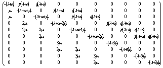 It then follows that
  | (14) |
where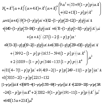
 and
and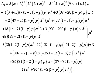
4. Availability Analysis of the System
4.1. Calculations for Configuration 1
For the availability case of configuration 1, the initial conditions for this problem are the same as for the reliability case. The differential equations forms can be expressed as
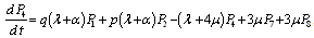 | , (15) |
 ,
, ,
, .This can be written in matrix form as
 | (16) |
where  is the coefficient matrix for the above equations.In the steady-state, the derivatives of the state probabilities become zero. This allows us to calculate the steady-state probabilities from
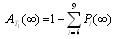 | (17) |
and | (18) |
Using the following normalizing condition: | (19) |
the above differential equations can be expressed as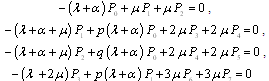
 | (20) |
 .Solving the system of equations (20) we obtain the steady-state probabilities
  in the availability case.For configuration 1, the explicit expression for
  is given by
 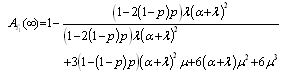 | . (21) |
4.2. Calculations for Configuration 2
Application of the above to configuration 2, with replacing in all equations, we obtain 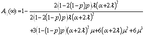 | (22) |
4.3. Calculations for Configuration 3
The differential equations can be expressed as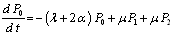 ,
, ,
, ,
, | (23) |
 .This can be written in matrix form as
 | (24) |
where  is the coefficient matrix for the above equations, Repeating the same steps as in configuration 1, it can be show that
 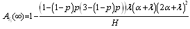 | (25) |
where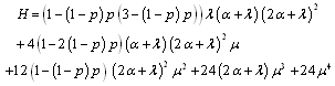
4.4. Calculations for Configuration 4
The differential equations can be expressed as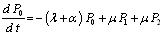 ,
,
 ,
, ,Equations
  , …,
, …,  are the same as their corresponding equations in configuration 3. The system of equations can be written in matrix form as
 | (26) |
where is the coefficient matrix for the above equations, Repeating the same steps as in the previous configurations, it can be show that 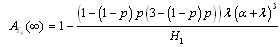 | (27) |
where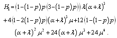 .
.
5. Special Cases
5.1. Study the Configurations When I.E. "Warm Standby becomes Cold Standby"
5.1.1. Calculations for Configuration 1
Mean time to system failure for configuration 1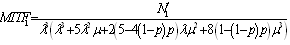 | (28) |
where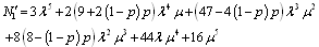 .Steady-state availability for configuration 1
 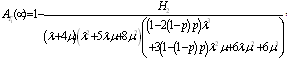 | (29) |
where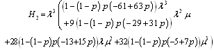 .
.
5.1.2. Calculations for Configuration 2
Mean time to system failure for configuration 2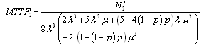 | (30) |
where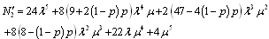 .Steady-state availability for configuration 2
 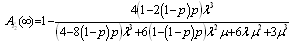 | . (31) |
5.1.3. Calculations for Configuration 3
Mean time to system failure for configuration 3 | (32) |
where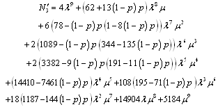 and
and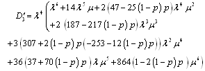 .Steady-state availability for configuration 3
 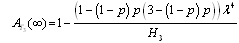 | (33) |
where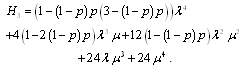 .
.
5.1.4. Calculations for Configuration 4
mean time to system failure for configuration 4 | (34) |
steady-state availability for configuration 4 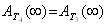 | (35) |
5.2. Study the Configurations When  I.E. "Warm Standby becomes Hot Standby"
5.2.1. Calculations for Configuration 1
Mean time to system failure for configuration 1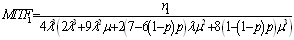 | (36) |
where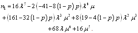 .Steady-state availability for configuration 1
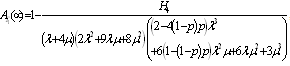 | (37) |
where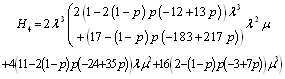 .
.
5.2.2. Calculations for Configuration 2
Mean time to system failure for configuration 2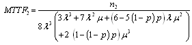 | , (38) |
where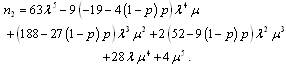 .Steady-state availability for configuration 2
 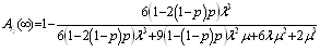 | . (39) |
5.2.3. Calculations for Configuration 3
Mean time to system failure for configuration 3 | (40) |
where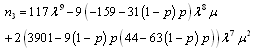
 and
and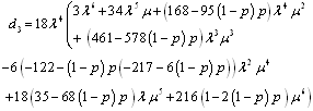 Steady-state availability for configuration 3
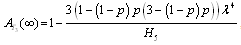 | , (41) |
where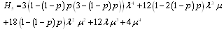 .
.
5.2.4. Calculations for configuration 4
Mean time to system failure for configuration 4 | (42) |
where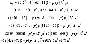 and
and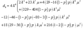 .Steady-state availability for configuration 4
 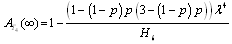 | (43) |
where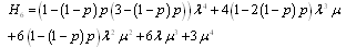 .
.
5.3. When  , the Results of All Configurations Reduce to Those Obtained by[7]
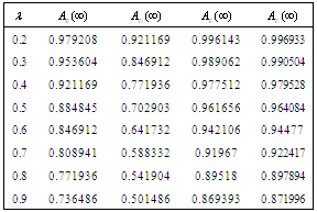
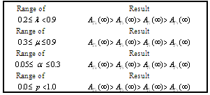
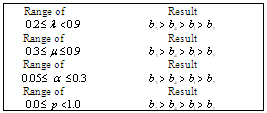
6. Comparison between the Four Configurations
The purpose of this section is to compare and  for
for  when
when  and
and  .
.
6.1. Comparisons for the  and
and 
Comparison of  and
and  , for
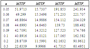
, for  , in the following three cases are illustrated in Tables (3-12)Case 1: fix
  ,
,  ,
,  and vary the values of
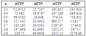
  . Case 3: fix
  ,
,  ,
,  and vary the values of
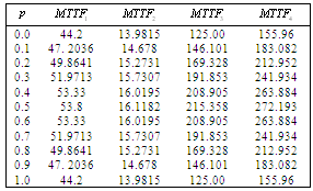
  .Case 2: fix
  ,
,  ,
,  and vary the values of
  . Case 4: fix
  ,
,  ,
,  and vary the values of
  .
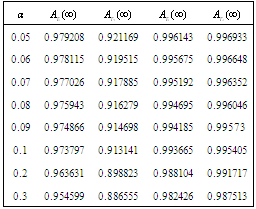
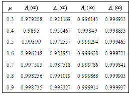
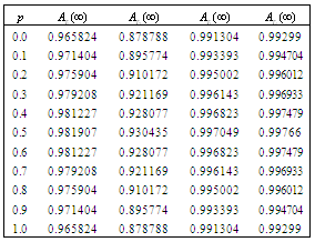
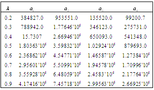
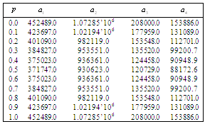
.Table 3. Comparison of
 by using four configurations when by using four configurations when
 , ,
 and and

 |
| |
|
Table 4. Comparison of by using four configurations when
 , ,
 and and

 |
| |
|
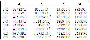
Table 5. Comparison of by using four configurations when
 , ,
 and and

 |
| |
|
Table 6. Comparison of by using four configurations when
 , ,
 and and

 |
| |
|
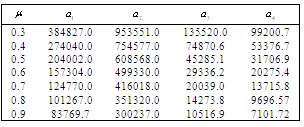
Table 7. Comparison of
 by using four configurations when by using four configurations when
 , ,
 and and

 |
| |
|
Table 8. Comparison of
 by using four configurations when by using four configurations when
 , ,
 and and

 |
| |
|
Table 9. Comparison of
 by using four configurations when by using four configurations when
 , ,
 and and

 |
| |
|
Table10. Comparison of
 by using four configurations when by using four configurations when
 , ,
 and and

 |
| |
|
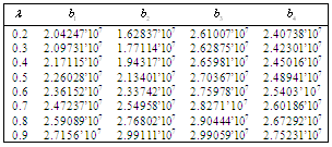
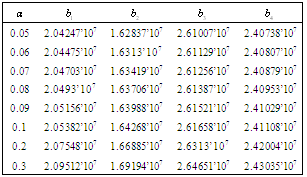
Table11. Comparison of configurations 1,2,3,4 for

 |
| |
|
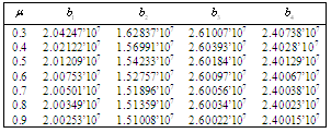
Table12. Comparison of configurations 1,2,3,4 for

 |
| |
|
6.2. Cost/ Benefit Ratio Comparisons
Let  and
and  where
where  is the cost for configurations i for
  which are listed in Table 2. Comparison of the
  and ,
and ,  in four cases, considered in section 6.1, are illustrated in tables (13-22).
Table 13. Comparison of by using four configurations when
 , ,
 and and

 |
| |
|
Table 14. Comparison of by using four configurations when
 , ,
 and and

 |
| |
|
Table 15. Comparison of by using four configurations when
 , ,
 and and

 |
| |
|
Table 16. Comparison of by using four configurations when
 , ,
 and and

 |
| |
|
Table 17. Comparison of
 by using four configurations when by using four configurations when
 , ,
 and and

 |
| |
|
Table 18. Comparison of
 by using four configurations when by using four configurations when
 , ,
 and and

 |
| |
|
Table 19. Comparison of
 by using four configurations when by using four configurations when
 , ,
 and and

 |
| |
|
Table 20. Comparison of
 by using four configurations when by using four configurations when
 , ,
 and and

 |
| |
|
Table 21. Comparison of configurations 1,2,3,4 for

 |
| |
|
Table 22. Comparison of configurations 1,2,3,4 for

 |
| |
|
7. Asymptotic Estimate of the Optimal Systems
Let  be a sample of failure times for operative units with
 be a sample of failure times for warm standby units with
 be a sample of repair times for failed units with
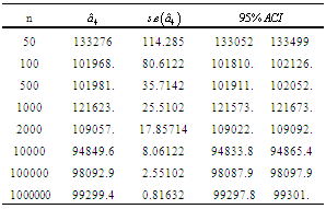
8.1. Asymptotic Estimate of Optimal Configuration 4
From Tables (11, 21), the optimal configuration, using the  measure is configuration 4. The estimate
  is defined by;
  | (44) |
where The asymptotic confidence interval ACI is given by
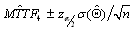 where
where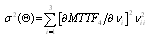 and
and 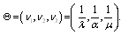
Table 23. ACI for
 , the true value , the true value

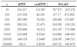 |
| |
|
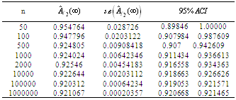
Table 24. ACI for
 , the true value , the true value

 |
| |
|
8.2. Asymptotic Estimate of Optimal Configuration 2
From Tables (12, 22), the optimal configuration, using the  measure is configuration 2. The estimate
  is defined by;
 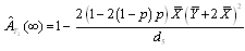 | , (45) |
where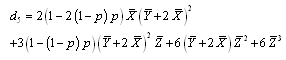 The asymptotic confidence interval ACI is given by
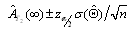 ,where
 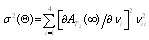 .
. Table 25. ACI for
 , the true value , the true value

 |
| |
|
Table 26. ACI for
 , the true value , the true value

 |
| |
|
8. Conclusions
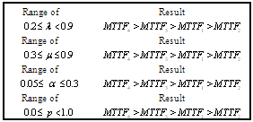
In this paper, we studied the mean time to system failure and the steady-state availability of four different series system configurations with mixed standby components. By comparing the  and
and  listed in Tables (3-10), Tables 11 and 12 are produced, from which the best configuration (highest
  and
and  ) is configuration 4. Tables 13-20 produce Tables 21 and 22, from which the optimal system based on (cost/benefit) measures (least
  and
and  ) are configurations 4 and 2 respectively. Asymptotic estimation of
  ,
,  and cost/ benefit are computed for the optimal systems. The numerical results of such asymptotic estimates are displayed in tables 23-26.
References
| [1] | M. Rashad, M. Salah El-Sherbeny, and Z. M. Hussien., Cost Analysis of a Two-unit Cold Standby System With Imperfect Switch, Patience Time and Two Type of repair, J. Egypt Math. Soc. 17 (1) (2009) 65-81. |
| [2] | Chandrasekhar, P., Natarajan, R. Confidence limits for steady state availability of a two unit standby system, Microelectronics Reliability, 34 (7) (1994) 1249-1251. |
| [3] | Chandrasekhar, P., Natarajan, R., Sheryl Sujatha, H., Confidence limits for steady state availability of systems, Microelectronics Reliability, 34 (8) (1994) 1365-1367. |
| [4] | Chandrasekhar, P., Natarajan, R., Confidence limits for steady state availability of a parallel system, Microelectronics Reliability, 34 (11) (1994) 1847-1851. |
| [5] | Chandrasekhar, P., Natarajan, R., Confidence limits for steady state availability of systems with lognormal operating time and inverse Gaussian repair time, Microelectronics Reliability, 37 (6) (1997) 969-971. |
| [6] | Chandrasekhar, P., Natarajan, R., and Yadavalli, V. S. S., A Study on a two unit standby system with Erlangian repair time, Asia-Pacific Journal of Operational Research, 21 (2004) 271-277. |
| [7] | Kuo-Hsiung Wang, Ching-Chang Kuo., Cost and probabilistic analysis of series systems with mixed standby components, Applied Mathematical Modelling, 24 12 (2000) 957-967. |
| [8] | Mahmoud, M.A.W. and Moshref.,. M.E., On a two-unit cold standby system considering hardware, human error failures and preventive maintenance, Mathematical and Computer Modelling, 51 (5) (2010) 736-745. |
| [9] | M. Salah El-Sherbeny., The optimal system for series systems with mixed standby components, Journal of Quality in Maintenance Engineering, 16 (3) (2010). |
| [10] | V.S.S. Yadavalli, A. Bekker, M. Botha, Asymptotic confidence limits for the steady state availability of a two-unit parallel system with 'preparation time' for the repair facility, Asia-Pacific Journal of Operational Research, 19 (2002) 249-256. |
| [11] | Wang, K.-H., Hsieh, C.-H., and Liou, C.-H., Cost benefit analysis of series systems with cold standby components and a repairable service station, Quality Technology & Quantitative Management, 3 (2006) 77-92. |
| [12] | Ying-Lin Hsu, Ssu-Lang Lee, Jau-Chuan Ke. A repairable system with imperfect coverage and reboot: Bayesian and asymptotic estimation, Mathematics and Computers in Simulation, 79 (2009) 2227-2239. |
 Abstract
 Reference
 Full-Text PDF
 Full-Text HTML