Rhonda Magel, Michael Hoffman
Department of Statistics, North Dakota State University, Fargo, United States
Correspondence to: Rhonda Magel, Department of Statistics, North Dakota State University, Fargo, United States.
| Email: |  |
Copyright © 2015 Scientific & Academic Publishing. All Rights Reserved.
Abstract
This research examines the salaries of Major League Baseball (MLB) players and whether players are paid based on their on-the-field performance. A random sample of players was selected for each season between 2010 and 2012. Models were developed to predict the salaries based on a variety of production statistics. Different models were created for position players and pitchers. Significant production statistics that were helpful in predicting salary were selected for each model. Two models were developed for position players and two models were developed for pitchers. One of the models in each group considered yearly production statistics and the other model considered career production statistics. The models which considered yearly production statistics could be used to determine whether or not a player was underperforming in comparison to his salary for that year. These models could not be used for predicting salary for the year since yearly production statistics are unknown ahead of time. The two models based on career production statistics were deemed to be good predictive models since their predictive r-squared values were at least 0.68. The regression models developed were tested for accuracy by predicting the salaries of a random sample of players from the 2013 MLB season.
Keywords:
Career Statistics, Yearly Statistics, Pitchers, Position Players, Stepwise Regression
Cite this paper: Rhonda Magel, Michael Hoffman, Predicting Salaries of Major League Baseball Players, International Journal of Sports Science, Vol. 5 No. 2, 2015, pp. 51-58. doi: 10.5923/j.sports.20150502.02.
1. Introduction
There has been an increasing amount of research on sports analytics and salary in particular. However, most of the research on salary has been conducted through analysing the length of a player’s contract and not on average yearly salary for a major league baseball (MLB) player. The goal of this study is to examine the significant factors for all players in determining average yearly salary. Different statistics need to be evaluated for pitchers and position players. Pitchers cannot be evaluated on the same statistics especially since pitchers in the American League do not bat. Separate models will be created for pitchers and position players. Indicator variables are used in the position player model to account for the different positions. These positions include: 1st baseman, 2nd baseman, 3rd baseman, shortstop, catcher, designated hitter, and outfielder. There was no differentiation made between the three outfield positions since many players played more than one outfield position throughout the season with little skill set differences between the outfielders. An indicator variable was also placed in the model for pitchers, differentiating between starting pitchers and relief pitchers. Starting pitchers may be paid more since a good starting pitcher would pitch 6 or more innings in a game while a relief pitcher is needed to hold the lead for an inning or two in a game (Gelb, 2012). Different types of relief pitchers were not accounted for in this study. Set-up pitchers and closers were grouped into the same position (relief pitchers).Two models are created for position players and two models are created for pitchers. The first set of models (one model for position players and one model for pitchers) use yearly statistics to try and account for the yearly salary of a given player for that season. The models using only yearly statistics are helpful in determining if players attained their expected production statistics for that year based on the salaries they were given. These models cannot be used for prediction since the yearly statistics a player receives are not known in advance. The second set of models developed, one model for position players and one model for pitchers, will try to predict the yearly salary of a baseball player based on the career statistics that a player has accumulated in prior seasons. In 2013, Major League Baseball (MLB) had 30 clubs divided over 2 leagues and 3 divisions per league. The baseball revenue for MLB was over 8 Billion dollars with a wide variety of different markets (“MLB team values”, 2014). A Revenue Sharing Plan was agreed to by the Major League Baseball Players Association in 2002 to help reduce some of the dominance of teams in larger markets. The MLB Revenue Sharing Plan has each team paying 34% of the Net Local Revenue into a “pool” of money. This “pool” of money is evenly distributed between all 30 teams. This allows for more equality between salaries of players based on their performance, regardless of their team (“Basic Agreement”, 2002).The MLB does not have a hard salary cap as in some sports such as the National Football League. Teams are allowed to spend as much as they please on salaries. However, the MLB tries to discourage overspending by the enforcement of the Competitive Balance Tax. Teams with a payroll over the threshold have to pay a penalty based on the number of consecutive years their payroll is above this threshold. (“Basic Agreement”, 2002). Only the New York Yankees have paid this tax every year and only 5 teams have ever paid a Competitive Balance Tax since it was implemented in 2003 (Axisa, 2013). This is important to note since in our analysis, we assume that players are in an open market and could get the same money throughout the league.There is a minimum salary in baseball and this has ranged between $400,000 and $500,000 between 2010 and 2014. This should not be a big factor in our analysis since rookies and players with less than 400 at-bats or 30 games pitched were excluded from our study. The maximum player salary for 2013 was $28,000,000 so there is a very wide range in salaries among players (Brown, 2012).Players are also allowed to have an arbitration hearing for their salary if they have between 3 and 6 years of playing time in the MLB. These players cannot become free agents or switch teams in this time period. This should not affect our models too much because it should be assumed that players will be able to get a competitive wage regardless of what team they play for due to the Revenue Sharing agreement and an open market (Axisa, 2013).
2. Past Studies
Moneyball (2011), a popular movie released in 2011 demonstrates the hard work that went into creating a roster on a limited budget for Billy Beane and the Oakland Athletics. In this movie, Billy Beane hires Peter Brand, a computer/statistical whiz, to use statistics to get the necessary production to be competitive and reach the playoffs while signing the players at a huge bargain. This movie is based on a true story of the 2002 Oakland Athletics where the Athletics were able to win 103 regular season games while only spending $39,679,746 which was the 3rd lowest payroll in the MLB in 2002. The Athletics had exactly the same number of wins as the New York Yankees in 2002, with the New York Yankees spending $125,928,583 which was the highest payroll in MLB in 2002 (Espn.com). Even though this was possible for Oakland, and a few teams try to get bargain players on a yearly basis, most teams in MLB have at least one player with a large contract indicating that if a team has a good player, they will try to keep them at almost any cost to keep the fans interested in the team (Orinick, 2014).Meltzer (2005) conducted one of the few studies looking at the average yearly salaries for position players only. In this study, Meltzer conducts a 2-stage least-squares regression by running two regression models; one model predicting the average yearly salary, and the other model predicting the length of contract. In these regression models, Meltzer (2005) uses the same independent variables for average yearly salary and length of contract. The models included two performance statistics; on-base plus slugging percentage (OPS), and plate appearances. The models also included other variable such as All-Star appearances, Gold Glove winnings, health status, age, position, contract status, and payroll for the team in which the player played for that season. After finding results for the first-stage regression models, Meltzer uses a two-stage regression predicting length of contract based on the average yearly salary found in first-stage regression model. He also predicted the average salary based on contract length found in the first-stage regression model. A subset of independent variables used in the first-stage regression models was also used in the second-stage regression model in addition to either the average salary or contract length estimated by the first-stage models. The study (Meltzer (2005)) found that “performance metrics are a significant predictor of player salary”. Hakes & Turner (2011) conducted a study on average yearly salary for position players based on age and on-base plus slugging percentage (OPS) along with several extraneous variables such as MVP awards, All-Star appearances, and Population of Market. They found that salary peaked at least 1.8 years after hitting productivity in baseball and salary declined slightly before retirement. It was also found that premier players had their performance decline slower than non-premier players.Stankiewicz (2009) examined the relationship between the length of a contract and the productivity of a player. Productivity was based on a weighted offensive statistic, Equivalent Average. This statistic, EqA, is similar to OPS except that EqA takes into account stolen bases whereas OPS is purely a power statistic. The main goal of Stankiewicz’s paper was to determine if players with long term contracts were actually more productive than players with one year contracts. It was found that players with long contracts (greater than 1 year) were in fact more productive and had a higher EqA. Stankiewicz’s research (2009) did not involve salary, but only length of contract.One final important study that was conducted in 2011, examined that effect of contract year performance and the future salary that the player received. Hochberg (2011) used data from 1993-2010 to examine the salary of position players. Hochberg’s study found that the performance of the player in the contract year was overweighted and the performance of the player in years previous to the contract year was underweighted in determining future salary. The position of a player was not found to be significant in determining salary (Hochberg (2011)).
3. Design of Study
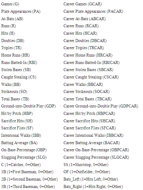
Data was collected from three MLB seasons which included the 2010, 2011 and 2012 seasons. Players with limited time in the major leagues were omitted. A player was omitted from the position player model if they had fewer than 400 at-bats. A player was omitted from the pitching model if they pitched fewer than 30 games. A restriction for the games pitched instead of innings pitched was used because innings per performance would not be equal for relief pitchers and starting pitchers. These thresholds were used because they accounted for approximately 1 full year of playing time for a full-time player. Since it was believed that salary might vary between the two leagues, a stratified random sample was used with 90 players selected from each league for both position players and for pitchers. This resulted in approximately 5-6 players on average from each team selected. The sample size was 540 players to develop the regression models (yearly and career) for position players and 540 pitchers to develop the regression models for pitchers. Salaries were collected from two different websites; Baseball Player Salaries (baseballplayersalaries.com), and Baseball Reference (baseball-reference.com). All the production statistics were then collected from Baseball Reference (baseball-reference.com). Some of the differentiations between starting pitchers and relief pitchers were found on the ESPN website (Espn.com).We examined many different production statistics instead of using only one or two production statistics, such as OPS or EqA, or plate appearances, as in previous studies. The statistics that were chosen were selected for two main reasons; Baseball fans were familiar with the statistics; and the statistics were easily accessible on the website baseball-reference.com. In order to adjust for the different variances in salary for a given set of production statistics and to make a better predictive model, the natural logarithm of salary was used for the dependent variable in all of the models. The batting statistics considered for entry into the position players models are given in Table 1 with yearly statistics considered for one model and career statistics used for the second model. The indicator variables considered for entry into both models are listed at the bottom of Table 1. The indicator variables indicated the position of the player and then whether they batted left or right handed. The pitching statistics considered for entry into the pitchers models are given in Table 2 with yearly statistics considered for one model and career statistics considered for the second model. A position indicator variable indicating whether the pitcher was a starting pitcher or a relief pitcher was also considered for both models. In order to help with model selection, the stepwise selection technique with an entry and exit alpha value of 0.15 was used to determine the initial set of significant variables in each model. Scatterplots of each significant predictor variable against log (salary) were graphed and a squared term was added to the model in relationships which appeared to be quadratic. This was due to findings of Hakes & Turner (2011) to possibly account for the decrease in salary at the end of one’s career. The final models were based on results from using stepwise regression plus adding the square terms of variables in which the relationship between the variable and the natural log of the salary appeared to be quadratic. Indicator variables representing the various positions were also included in the models if at least one of the indicator variables for a position was significant. Once the models were developed, a stratified random sample was taken consisting of 90 position players from each league and 90 pitchers from each league in 2013. The sample of position players is used to test the position player models and the sample of pitchers is used to test the models for pitchers.Table 1. Batting Statistics Considered
 |
| |
|
4. Results
4.1. Yearly Position Player Model
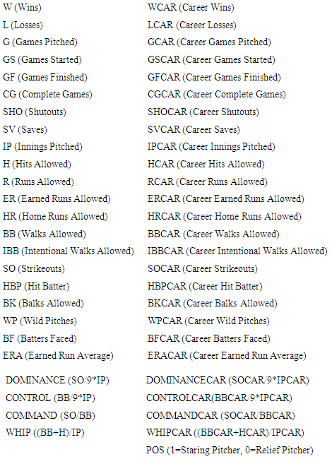
The first model that was developed was a model for the salary of a position player based on their performance statistics for that given year. This model could be used to see if players are performing in accordance to their salary. The variables considered for entry into this model using stepwise regression are given on the left side of Table 1 down to and including slugging percentage. As stated in section 3, each variable found significant in the model through the stepwise regression technique was plotted against the natural log of the salary. If this plot appeared to be quadratic, a square term of the variable was also added to the model. Table 2. Pitching Statistics Considered
 |
| |
|
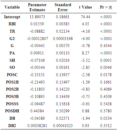
Using the technique outlined in Section 3, the performance statistics included in this model were the following: Runs Batted In (RBI), Triples (TR), Games (G), Games Squared (G2), Plate Appearances (PA), Sacrifice Hits (SH), Strikeouts (SO), Doubles (DB) and Doubles Squared (DB2). The position indicators were also included in the model since at least one of the indicator variables were found to be significant. These included Catcher-POSC, 1st baseman-POS1B, 2nd baseman-POS2B, 3rd baseman-POS3B, shortstop-POSSS, designated hitter-POSDH, and if all indicator variables for position are 0 this would be outfielder. The model results are given in Table 3. The year (2010, 2011, or 2012) was not found to be significant. The model (given in Table 3) was significant in explaining yearly salaries of position players with an overall F statistic value of 19.17 based on 15 and 524 degrees of freedom and p-value less than 0.000. The standard residual error for the model was 0.9862 based on 524 degrees of freedom. A residual plot was graphed for natural of y versus the residuals and the assumptions of the model appeared to have been met. It is noted that the indicator variables for year (2010, 2011, or 2012) were not included in Table 3 because they were found not to be significant. Even though the model was found to be significant in explaining the variation in yearly salaries of position players, it does not appear to be a very good model since only 35% of the variation in salaries is explained by this model (R2). The adjusted R2 value for the model was 0.336. The model does not account for the health or injury of a player. In baseball, the performance of a player from year to year is variable. It is common in even premier players to have a bad year once in a while. Players could have a change of 10 homeruns from one year to another or have their batting average drop or increase by 0.04 in a year, which would affect the salary prediction significantly. Using this model, 261 players had a negative residual (underpaid according to yearly statistics) and 279 players had a positive residual (overpaid).Table 3. Yearly Position Players Model Output
 |
| |
|
4.2. Yearly Pitchers Model
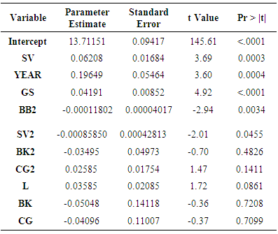
A model similar to the yearly position player model was developed for pitchers. This yearly model can be helpful in determining if pitchers are performing close to their expectations. In this case, the dependent variable is the natural logarithm of the salary. The stepwise selection technique was used to determine the significant yearly production statistics in this model with an alpha level of 0.15 for both entry and exit into the model. Residual plots were then conducted. Higher order terms were added to the model if indicated by the residual plots as outlined in Section 3. The yearly performance statistics in the model included: saves (SV), saves squared (SV2), year (YEAR), number of games started (GS), walks allowed (BB), walks allowed squared (BB2), balks (BK), balks squared (BK2), number of losses (L), number of complete games(CG), and number of complete games squared (CG2). This model was developed based on a sample size of 539 since one observation (James Shields in 2011) was deleted from the sample because of a large Cook’s Distance (Abraham & Ledolter, 2006). The model results are given in Table 4. The model was significant at helping to determine salaries of pitchers based on an overall F-statistic value of 17.66 with 10 and 528 degrees of freedom. The p-value was less than 0.0001. The residual standard error was 0.4472 based on 528 degrees of freedom. A plot of the natural logarithm of the salary versus the residuals for this model indicated that model assumptions were being met. Table 4. Yearly Pitchers Model Output
 |
| |
|
Even though the model is significant, it is not a very good model for predicting salary, since it only explains approximately 25% of the variation in salary (R2). The adjusted R2 value for the model is 0.2364. Using the model, 263 pitchers have negative residuals (underpaid) and 276 pitchers have positive residuals (overpaid). Therefore, there does not appear to be a large difference in the number of players being overpaid or underpaid, but a wide spread in performance and salary. The findings support the opinion of other researchers who were reluctant to model pitcher’s salary because of the extreme differences in pitcher statistics due to their role in the game (Meltzer, 2005) since there is a wide variation as to how pitchers are used.. Our model did not find the position variable (starting or relief pitcher) as being significant.
4.3. Career Position Players Model
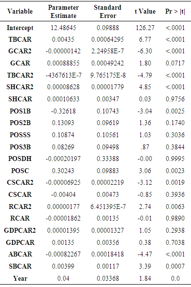
In the next phase of model development, we used the career statistics of a position player in an effort to develop a model to help predict the player’s salary. Yearly statistics for each player in the model were aggregated from 1984 to the year before the player’s salary was examined. If a player’s salary was examined in 2010, the career statistics were aggregated up to 2009 for that player. The same production statistics that were considered for the year were considered for the entire career for each player. These are given in Table 1. Stepwise regression with an alpha level of 0.15 for entry or exit was used initially to help develop the model. Following the technique as outlined in Section 3, residual plots were graphed against each of the independent variables found significant using stepwise. Quadratic term of variables were added to the model as a result of these residual plots and tested for significance. They were left in the model if they were found to be significant. The final set of significant career production statistics were the following: total bases (TBCAR), total bases squared (TBCAR2), games (GCAR), games squared (GCAR2), sacrifice hits (SHCAR, sacrifice hits squared (SHCAR2), position (POS1B, POS2B, POSSS, POS3B, POSDH, POSC), caught stealing (CSCAR), and year (YEAR). The regression output is found in Table 5 for this model. In this model, the position of the player was found to be significant as well as the year. It makes sense that year would be significant because salaries could increase each year due to inflation. The results from this model indicate that some positions demand higher salaries than other positions. Recall that in the yearly model, year and position were not significant. Table 5. Career Position Players Model Output
 |
| |
|
There were four players found in which Cook’s Distance values associated with these four players was large. The observations for these four players were eliminated from the model to remove any bias in our estimates (Abraham & Ledolter (2006)). The regression model was then developed based on a sample of 536 observations. The overall F-statistic for the model was 70.51 with 21 and 514 degrees of freedom with a residual standard error of 0.2727. The model significantly helps to explain the variation yearly salaries of position players with a p-value of less than 0.0001. A plot of the residuals versus the predicted values indicated that the model met the assumptions with constant variance. The model had an R-squared value of 0.7423 and an adjusted R2 value of 0.7318. The predicted R-squared value associated with this model was 0.7155, which indicates that the model should do a fairly good job at predicting salaries of position players.
4.4. Career Pitchers Model
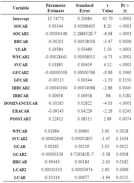
A regression model was developed to model the natural logarithm of pitcher’s salaries based on their career statistics. The pitching statistics given in Table 2 based over the career of a player were considered for entry into the model. Stepwise regression with an alpha of 0.15 for entry and exit was conducted to derive the initial model. Higher order terms for the variables in the initial model were considered as indicated by residual plots and then tested for significance. The following career statistic variables were found to by significant: strike outs (SOCAR), strike outs squared (SOCAR2), walks (BBCAR), wild pitch (WPCAR), wild pitch squared (WPCAR2), saves (SVCAR), saves squared (SVCAR2), games finished (GFCAR), games finished squared (GFCAR2), intentional walks (IBBCAR), intentional walks squared (IBBCAR2), dominance (DOMINANCECAR), earned run average (ERACAR), games (GCAR), games squared (GCAR2), home runs allowed (HRCAR), losses (LCAR), losses squared (LCAR2), year (YEAR), and pitcher role (POSSSTART). The model is given in Table 6.Table 6. Career Pitchers Model Output
 |
| |
|
Observations associated with two players had high Cook’s distances. These players were Mariano Rivera in 2011 and Billy Wagner in 2010. Both of these players were in the last couple of years of their career and previous research has indicated this could be a problem in predicting salaries. The observations associated with these players were eliminated since they did have high Cook’s distances in order to reduce any bias in the regression coefficients. The regression model was then estimated with a sample of 538 observations. The model had an F value of 63.2 with 20 and 517 degrees of freedom indicating the model was significant at explaining yearly salaries of pitchers based on a p-value of less than 0.0001. The residual standard error for the model was 0.2803 and the residual plot indicated that the assumption of constant variance was satisfied. The model had an R-squared value of 0.7097 and an adjusted R2 value of 0.6985. The predicted R-squared value for this model was 0.6872. This model does have a lower predicted R-squared value than the career position model, but it should still be able to do a reasonable job in predicting a pitcher’s salary based on their previous career statistics. Pitchers do have several varying roles and sometimes their role is switched during the season. This could be the reason for the lower R-squared value.
5. Prediction
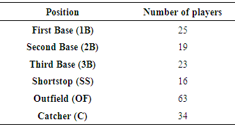
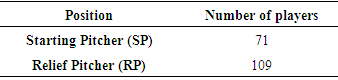
The two models, one for position players and one for pitchers, based on a player’s career statistics were used to see how well they could predict 2013 baseball salaries. A stratified random sample of 90 players from each league was sampled for both the model for the pitchers and the model for the position players. This random sample yielded 180 players for each model to be used to predict the salaries. The number of players selected from each position in this sample for position players and pitchers is given in Tables 7-8. No one in the designated hitter position was selected for the sample. This occurred by random chance due to the limited number of players in this position. Table 7. Number of Position Players by Position in 2013 Dataset
 |
| |
|
Table 8. Number of Pitchers by Role in 2013 Dataset
 |
| |
|
5.1. Predictions for Position Players
The salary predictions for position players are based on the career statistics of the player before 2013. The dependent variable in the regression model was the natural logarithm of the salary to adjust for unequal variances in salaries when the career statistics are held constant. We will give an example as to how this model was used in making predictions of salaries. Joe Mauer’s (catcher) career statistics before 2013 are as follows: TBCAR=1839; GCAR=1065; SHCAR=4; CSCAR=15; RCAR=626. In order to find his predicted salary for 2013, you would multiply each estimated regression parameter by the corresponding career statistic and add these together (see Table 5). In this case, we would have the following: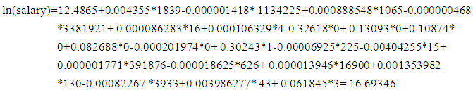 Joe Mauer’s actual salary in 2013 was 16.95100 on the natural logarithm scale. The error (actual-predicted), in this case was16.951-16.69346 = 0.25754
 Table 9. Accuracy of Position Player Predictions
 |
| |
|
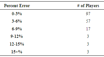
The Percent Error compared to the actual salary is the absolute value of the error divided by the actual salary times 100. The Percent Error in the natural log scale is given below:Percent Error = [actual salary-predicted salary]/actual salary X 100 = [0.25754]/16.951 X 100=1.52%The Percent Error was found for all the 180 position players in the 2013. All but 9 players had a Percent Error of less than 9%. The model was doing a fairly good job at predicting the natural logarithm values of their salaries given their career statistics that were found to be significant in the model. The results are given in Table 10.
5.2. Predictions for Pitchers
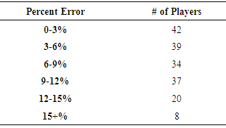
The prediction of the natural logarithm for a pitcher’s salary is based on the career statistics of the player before 2013. As an example as to how this model is used, we considered the career statistics of C.C. Sabathia before 2013. The career statistics of C.C. Sabathia (starting pitcher) before 2013 are as follows: SOCAR=2235; BBCAR=767; SVCAR=0; GFCAR=0; IBBCAR=31; DOMINANCECAR = 0.86722; ERACAR=4.773; GCAR=385; HRCAR=229; LCAR=104; POSSTART=1.In order to find C.C. Sabathia’s predicted salary for 2013, we multiplied each estimated parameter by the associated career statistics and obtained the ln(salary) estimate of 17.03726. The actual salary for C.C. Sabathia in 2013 was 16.951 on the natural log scale. The error in this case was16.951-17.03726 = -0.08626Percent Error = [ 0.08626 ]/16.951 X 100=0.51%The accuracies of all of the 180 predictions for pitchers are given in Table 10.Table 10. Accuracy of Pitcher Predictions
 |
| |
|
6. Conclusions
After fitting models and predicting the salaries of random samples of position players and pitchers, it was found that the models using career production statistics were the most useful for both pitchers and position players since these statistics are known in advance of signing a player to a contract. Several career production statistics were included in both models. The significant career performance statistics for position players included: Total Bases, Total Bases Squared, Games, Games Squared, Sacrifice Hits, Sacrifice Hits Squared, Position, Caught Stealing, Caught Stealing Squared, Runs, Runs Squared, Ground into Double Play, Ground into Double Plays Squared, At-Bats, and Stolen Bases. A different subset of performance statistics was found to be significant in determining the salaries of pitchers which included: Strike Outs, Strike Outs Squared, Walks, Wild Pitch, Wild Pitch Squared, Saves, Save Squared, Games Finished, Games Finished Squared, Intentional Walks, Intentional Walks Squared, Dominance, Earned Run Average, Games, Games Squared, Pitcher Role, Home Runs Allowed, Losses, and Losses Squared. The career performance statistics led to a high predictive power in determining salaries as the predictive R-squared values were 0.7155 and 0.6872 for the position players and pitchers, respectively. After developing the models to predict salaries for both pitchers and position players, predictions of salaries were made for a random sample of 180 pitchers and a random sample of 180 position players. It was found that prediction errors for the natural logarithm of salary were within 0% to 12% for approximately 84% of the pitchers and approximately 96% for position players. Therefore, career production statistics appear to explain a lot of the variation in salaries. It was also found that players in the last few years of their career did not fit the model very well since these players were paid either lower than their career statistics would indicate or paid higher than their career statistics would suggest due to fan popularity and mentorship they could offer to younger players on the team. Examples of these players included Mariano Rivera and Billy Wagner. Health status variables and number and type of awards won were not considered in the models. It might be beneficial to look into All-Star game appearances, Most Valuable Player (MVP) awards, Gold Glove awards, and possibly the number of days on the disabled list in their career. Award winnings will likely increase the salary of these players significantly but also only apply to a relatively small portion of players. Research could examine the effect of performance bonuses for players. Many players today sign a contract with incentives to produce certain performance. It would be interesting to see if these contracts significantly increase the production statistics for these players or if it is better not to have contracts of this type.
References
| [1] | Abraham, B., & Ledolter, J. (2006). Introduction to regression modeling. Belmont, California: Thomson Brooks/Cole. |
| [2] | Axisa, M. (2013, September 11). Report: Yankees set to pay record $29.1 million luxury tax bill. Retrieved from http://cbssports.com/mlb/eye-on-baseball/23592770/report-yankees-set-to-pay-record-291-million-luxury-tax-bill. |
| [3] | Basic agreement. (2012). Retrieved fromhttp://mlb/mlb.com/pa/pdf/cbs_english.pdf. |
| [4] | Baseball player salaries. (2014). Retrieved from http://baseballplayersalaries.com/. |
| [5] | Baseball-reference. (2014). Retrieved from baseball-reference.com. |
| [6] | Brown, M. (2012, June 04). Bizball. Retrieved from http://www.baseballpropectus.com/article.php?articleid=17225. |
| [7] | Espn. (2014). Retrieved from Espn.com. |
| [8] | Hakes, J.K. & Turner, C. (2011) Pay, productivity and aging in major league baseball. Journal of Productivity Analysis. 35, 61-74. |
| [9] | Hochberg, Daniel. “The Effect of Contract Year Performance on Free Agent Salary in Major League Baseball” 2011, Department of Economics, Haverford College. |
| [10] | Gelb, M. (2012, 09 11). Understanding payroll and luxury tax. Retrieved fromhttp://www.philly.com/philly/blogs/phillies_zone?unerstanding-payroll-and-luxury-tax.html. |
| [11] | Meltzer, Josh. “Average Salary and Contract Length in Major League Baseball: When Do They Diverge?” 2005, Department of Economics, Stanford University, CA. |
| [12] | Mlb salaries. (2014). Retrieved fromhttp://www.cbssports.com/mlb/salaries. |
| [13] | Mlb team values. (2014) Retrieved fromhttp://www.forbes.com/mlb-valuations/list/. |
| [14] | Orinich, S. (2014). Mlb team payrolls. Retrieved from http://www.stevetheump.com/Payrolls.htm. |
| [15] | Stankiewicz, Katie (2009) “Length of Contracts and the Effect on the Performance of MLB Payers,” The Park Place Economist: Vol. 1. |
 Abstract
 Reference
 Full-Text PDF
 Full-text HTML