WentingWang, Rhonda Magel
Department of Statistics, North Dakota State University, Fargo, ND 58108, USA
Correspondence to: Rhonda Magel, Department of Statistics, North Dakota State University, Fargo, ND 58108, USA.
| Email: |  |
Copyright © 2014 Scientific & Academic Publishing. All Rights Reserved.
Abstract
There has been much attention paid to predicting the winner of the NCAA Men’s Basketball Tournament each year. In this research, we concentrated on deriving a method to predict the winner of the NCAA Women’s Basketball Tournament. Various models were developed to predict winners in each round using data from the 2011 and 2012 tournaments to develop these models. The models selected were verified using data from the 2013 tournament, and then used consecutively to predict the results from the 2014 tournament before any games were played. The variables found to be significant in developing the models included the differences in the following seasonal variables: field goal percentage; average number of assists per game; average number of steals per game; average number of points scored per game; average percentage of 3 point goals made; average percentage of free throws made; average number of blocks per game; and seed numbers. The point spread models, when used continuously from rounds 1 through 6, had a correct prediction percentage of 76% in 2014, and correctly predicted all four teams making it to the final four, the two teams in the championship game, and the winner.
Keywords:
Least squares regression models, Logistic regression models, Point spread, Probability of winning
Cite this paper: WentingWang, Rhonda Magel, Predicting Winners of NCAA Women’s Basketball Tournament Games, International Journal of Sports Science, Vol. 4 No. 5, 2014, pp. 173-180. doi: 10.5923/j.sports.20140405.04.
1. Introduction
The National Collegiate Athletic Association (NCAA) Women’s Division I basketball tournament is an annual collegiate basketball tournament for women held every spring during March and April. It was inaugurated during the 1981-82 season. In 2003, the final women’s championship game was moved to the Tuesday following the Monday men’s championship game. This means the women’s championship game is now the final overall game of the college basketball season. Unlike the men’s tournament, the women’s tournament has no play-in games. There are a total of 64 teams playing in the tournament, of which 31 of the teams are automatic bids. The remaining teams are granted “at-large” bids by the NCAA Selection Committee [1].The tournament is split into four regional tournaments including Midwest, West, East and South. Each regional tournament has teams seeded from 1 to 16. The teams having seeds summing up to 17 in each region, play each other during the first round. Teams winning in the first round, advance to the second round, and teams losing are eliminated. There are a total of six rounds in the tournament referred to as Round 64, Round 32, Sweet 16, Elite 8, Final 4, and Championship, respectively [1]. We will begin by mentioning some of the research related to the men’s NCAA Division I tournament. Carlin [2] considered regression models to estimate the probability of a team winning a game in the men’s NCAA tournament by using seed positions and computer ranking. Schwertman, Schenk, and Holbrook [3] modified the approach to fit linear and logistic regression models as a function of the difference in either team seeds or normal scores of the team seeds. Smith and Schwertman [4] developed more complex regression models to help predict point spread using the seed values. Caudill [5] developed a maximum score estimator based on seed values. Kubatko, Oliver, Pelton and Rosebaum [6] analysed correlations and relationships among various in-game basketball statistics. West [7] used ordinal logistic regression and expectation to estimate the probabilities that a given team would win 0 games through to 6 games. Zhang [8] modified the work of West and developed a conditional logistic probability model that outperformed West’s model in the 2013 NCAA men’s basketball tournament. In Zhang’s model, the probabilities of all teams that are up against each other trying to get to a particular spot in the tournament making it to that spot in the tournament add up to 1. In West’s model, the probabilities do not add up to 1, presenting an unrealistic situation since only one of the teams can make it to that spot in the tournament. Magel and Unruh [9] analyzed NCAA Men’s basketball games and found four common statistics were significant in determining which team won the game. These four common statistics included assists, free throw attempts, defensive rebounds, and turnovers. It is hard to find articles related to predicting NCAA women’s basketball games. This may be because research has shown that men’s sports draw a lot more attention even though the number of women and girls actively participating in sports has increased ([10] and [11]). This paper will concentrate on developing models to predict the team winners in future NCAA Women’s Basketball Tournaments.
2. Description of Study
The research objectives for this study were the following:1. Develop least squares regression models to estimate the point spreads of basketball games for Round 1, Round 2, and then Rounds 3-6 of the NCAA Women’s Basketball Tournament; and use these models to predict the winners of each game of the tournament and then the championship game. And2. Develop logistic regression models for Round 1, Round 2, and Rounds 3-6 to estimate the probability of a given team winning each of the games; and use these models to predict the winners of each game of the tournament and then the championship game.There were three phases of this study. During the first phase, models were developed. Data to develop the models was collected from the 2011 and 2012 NCAA Women’s Basketball tournament and using the seasonal averages of teams making it to the tournament. Seasonal averages were collected for all teams playing in the 2011 and 2012 tournaments on the following 8 variables: Field Goal Percentage; 3-pt Goal Percentage; Free Throw Percentage; Number of Rebounds; Number of Assists; Number of Blocks; Number of Steals, and Number of Points per game. The seed number that each team was given in either the 2011 or 2012 tournament was also noted. These variables were used because they are readily available on the NCAA website and many of them have been found to be significant in determining the winner of Men’s NCAA Basketball games. The first model developed estimated point spread of round 1 games. This was based on a sample size of 128 and included data from teams playing in the first rounds of both the 2011 and 2012 tournaments. The second model estimated point spread of round 2 games. This model was developed based on a sample size of 64 which included data taken from teams playing in the second round of the 2011 and 2012 tournaments. The third model estimated the point spread of games in the remaining rounds. This model is based on a sample size of 60 which included data taken from teams playing in the third through final rounds of the tournaments in 2011 and 2012.Logistic regression was also used to develop three different models. The first model estimated the probability of a team playing in the first round of winning the game. The second model estimated the probability of a team playing in the second round of winning the game. The third model estimated the probability of a team winning the game in round k if they made it to round k where k was equal to 3, 4, 5, or 6. The same variables considered for the point spread models were considered for these models. The sample sizes used to develop the logistic models were the same as the sample sizes used to develop the point spread models.The second phase of the study involved validating the point spread and logistic models. In order to do this, a different data set was used, namely data collected from the 2013 tournament. Seasonal averages of the variables found significant in any of the models were collected on all teams playing in the 2013 tournament. The first set of models were validated by using seasonal data collected on teams playing in the in the first round and placing the values from this data in the first round models and determining which team was predicted to win according to the model (either point spread or logistic). The predictions were compared to the actual results. The second set of models were validated by using seasonal data collected on teams playing in the second round of the tournament. The data values for teams playing against each other in the second round of the tournament were placed in the model (either point spread or logistic) and a winner was predicted using the model for each game in the second round. These predictions were compared to the actual results. The same process was followed using the models developed for round 3 through the final round. Predictions from the models were compared to the actual results. A model was considered to be validated if the model correctly predicted at least 67% of the games correctly in that set of rounds.The third phase of the study involved bracketing the entire set of games from the 2014 tournament and predicting a winner based on the point spread models developed. Seasonal averages of the variables found to be significant in the models were collected on all teams playing in the tournament. The first set of models developed were used to predict winners of the first round. Data from teams predicted to win the first round were place in the models developed for the second round. Winners from the second round were predicted based on the second round model and the data from the teams predicted to win the second round were placed into the third round model and predictions were made based on this model. Data from teams predicted to win the third round were placed into the model for the 4th round and predictions were made. Data from teams predicted to win the 4th round were placed into the model for the 5th round and predictions made. Data from the two teams predicted to win the 5th round was placed into the final round model and a prediction was made as to the winner of the tournament.
2.1. Developing Models for the First Round
The response variable for the ordinary least square regression model was point spread in the order of the team of interest minus the opposing team. A positive point spread indicates a win for the team of interest and a negative value indicates a loss for the team of interest. There were 128 teams playing 64 games in the first round of the tournaments in 2011 and 2012. For the 32 games in the first round of 2011, the point spread was obtained by using the scores of weaker teams (higher seed numbers) minus the scores of stronger teams (lower seed numbers). For the 32 games of the first round of the tournaments in 2012, the point spread was acquired by using the scores of stronger teams (lower seed numbers) minus the scores of weaker teams (higher seed numbers). The intercept was excluded when developing the models because the models should give the same results regardless of the ordering of the teams in the model. Therefore, it should not matter which team is considered first. Stepwise selection was used with an alpha value of 0.15 for both entry and exit to develop the models. The differences between the seasonal averages for the variables of the two teams playing in the game were considered for entry into the model. The variables under consideration included the following: Field Goal Percentage; 3-pt Goal Percentage; Free Throw Percentage; Number of Rebounds; Number of Assists; Number of Blocks; Number of Steals, and Points per game. The differences between seeds were also considered. The stepwise process started with no variables in the model, entered the variable that was most significant with point spread, checked to see if this variable was significant, entered the next variable that was most significant with the one variable already in the model if the first variable was significant, checked to see if the new variable entered was significant and checked whether the original variable entered was significant with the new variable in the model, otherwise the original variable was taken out of the model. This stepwise process continued finding the next variable that was most significant with point spread with the other variables in the model. If the new variable was significant, it was kept in the model, and the other variables in the model were considered with the variable with the largest p-value tested for significance with the new variable in the model and this variable was eliminated from the model if it was not significant. The process stopped if the new variable entered was not significant and was taken out of the model. The backwards selection procedure was also used with an alpha level of exit equal to 0.10. This process started with all of the variables in the model, tested the variable for significance with the largest p-value and took this variable out of the model if it was not significant, refit the model, tested the variable for significance that had the largest p-value. The process stopped if the variable that had the largest p-value was significant; otherwise, the variable was taken out of the model, the model refit, and the process repeated. The backwards regression process gave similar results to the models obtained from the stepwise regression process. The models from the stepwise regression process were used for predictions. In the few cases where the stepwise and backwards models may have varied, the r-squared values and predicted r-squared values were very similar. Model assumptions for the model were verified by using residual plots. The error terms did appear to be approximately normally distributed with constant variance [12].A logistic model [12] was also developed for the first round estimating the probability that the team of interest will win the basketball game. The response variable for this model was recorded as “1” if the team of interest won the game and as a “0” if the team of interest lost the game. No intercept was used during the development of the logistic model because the ordering of the teams in the model should not matter. Stepwise selection (as described in the previous paragraph) was used with an alpha value of 0.15 for both entry and exit when determining the significant variables for this model. The same differences of the seasonal averages for both teams used in the ordinary least squares regression model were considered for this model in addition to the seed differences. The Hosmer-Lemeshow (HL) test was conducted to determine whether the logistic model was appropriate. The p-value for the HL test was 0.907 indicating that there was no evidence to indicate the logistic model was not a good fit.
2.2. Developing Models for the Second Round
There were 64 teams playing 32 games in second rounds of the tournaments in 2011 and 2012. For the 16 games of the second round in 2011, the point spread was obtained by using the scores of the weaker teams (higher seed numbers) minus the scores of stronger teams (lower seed numbers). For the 16 games of the second round in 2012, the point spread was obtained by using the scores of stronger teams (lower seed numbers) minus the scores of weaker teams (higher seed numbers). The intercept was excluded when developing the model. The differences between the seasonal averages of the two teams for the variables mentioned were considered for entry into the model as well as the differences between the seeds of the teams.A logistic model was also fit for each game in the second round of both the 2011 and 2012 tournaments with the response variable being “1” if the team of interest won the game and “0” if the team of interest lost the game. No intercept was used.
2.3. Developing Models for the Third and Higher Rounds
There were 60 teams playing 30 games in the third and higher rounds of the tournaments in 2011 and 2012. For the 15 games of the third and higher rounds in 2011, the point spread was obtained by using the scores of weaker teams (higher seed numbers) minus the scores of stronger teams (lower seed numbers). For the 15 games of the third and higher rounds in 2012, the points spread was obtained by using the scores of the stronger teams (lower seed numbers) minus the scores of weaker teams (higher seed numbers). The intercept was excluded when developing the model. Stepwise selection was used with an alpha value of 0.15 for entry and exit. The differences between the seasonal averages of the two teams for the previously mentioned variables were considered for entry into the model as well as the differences between the seeds.A logistic model was also fit using the same initial variables considered as in the third and higher round point spread model with the response variable being “1” if the team of interest won the game and “0” if the team of interest lost the game. Stepwise selection was again used with an alpha value of 0.15 for a variable to enter or exit the model.
2.4. Steps Used for Verifying the Models
Using the ordinary least squares regression model developed to estimate the point spread of first round basketball games, the point spreads of the 32 games in the first round of the 2013 tournament were estimated. Values from the 2013 season of the variables found to be significant in the model were placed into the model for one game and the estimated point spread,  was obtained. If
  a predicted win for the team of interest using the point spread model was coded.If
  a predicted loss for the team of interest using the point spread model was coded.Using the logistic regression model developed to estimate the probability of the team of interest winning the game, this probability was estimated for the 32 games in the first round of the 2013 tournament. If the probability was estimated at 0.50 or higher, the team of interest was predicted to win the game. Otherwise, the opposing team was predicted to win the game. The second round and then the 3rd and higher rounds ordinary least squares regression models and logistic regression models were verified in a similar way, using the 32 teams that actually made it to the second round, the 16 teams that actually made it to the third round and so on. Namely, the models were verified using round by round results.
2.5. Steps Used for Bracketing and Prediction
In an effort to determine how well the ordinary least squares models did at prediction, we used the results from the models to complete our women’s bracket for the 2014 NCAA basketball tournament. Once the set of 64 teams was determined in 2014, we applied the model developed for round 1 to each of the 32 games in an effort to estimate the point spread and predict a winner of each of these games. We then placed the predicted winning teams in the round 2 model, estimated the point spread for these 16 games, and predicted the winners of round 2. The predicted winners in round 2 were then placed in the model developed for round 3. The point spread for each of these 8 games was estimated and winners were predicted for this round. The model was then used again using the predicted winners of round 3, in order to predict the winners of round 4. This process continued until a champion was predicted.
3. Results
3.1. Models Developed for First Round
The model developed to predict point spread of games played in the first round using ordinary least squares regression was found to be: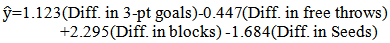 | (1) |
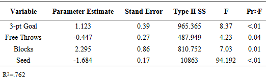
The standard errors and p-values associated with each of the parameter estimates for the model are given in Table 3.1. The associated R-square values as variables are added to the model are also given in the table. The model will all four variables explains an estimated 76% of the variation in point spread (R-square=0.762). The adjusted R-square value was 0.746.Table 3.1. Point Spread Model Parameter Estimates
 |
| |
|
The logistic model developed to help estimate the probability of the team of interest winning the game for teams playing in the first round of the playoffs was found to be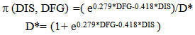 | (2) |
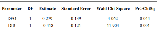
Where π (DIS, DFG) is the estimated probability that the team of interest will win the game with difference in seed, DIS, and difference in field goal percentage, DFG, in model.Table 3.2 gives the parameter estimates, their standard errors and associated p-values. The Hosmer and Lemeshow test was done to test whether there was evidence the logistic model was not appropriate. The p-value was 0.907 indicating that there was no evidence to reject using the logistic model.Table 3.2. Logistic Regression Model Parameter Estimates
 |
| |
|
3.2. Models Developed for Second Round
The model developed to predict point spread of games in the second round is given by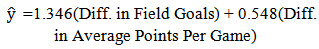 | (3) |
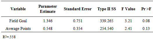
The standard errors and F values associated with each of the parameter estimates for the model are given in Table 3.3. The model with the two variables found to be significant explains about 56% of the variation in point spread (R-square=0.558). The adjusted R-square value was 0.529.Table 3.3. Point Spread Model Parameter Estimates
 |
| |
|
The logistic model developed to estimate the probability that the team of interest would win the game in the second round of the tournament was found to be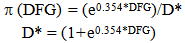 | (4) |
Where (DFG) is the estimated probability that the team of interest will win the game. The only variable that was significant in this model was the difference in field goal percentage, DFG, which had a p-value less than .002. The Hosmer and Lemeshow Goodness of Fit test was performed to test if the logistic model was appropriate. There was insufficient evidence to indicate the logistic model was not appropriate since the p-value was 0.3354.
3.3. Models Developed for Third and Higher Rounds
The point spread model developed to estimate the point spread of games in the third and higher rounds was found to be: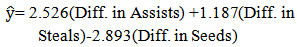 | (5) |
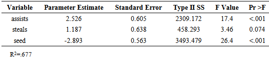
The standard errors and p-values associated with each of the parameter estimates for the model are given in Table 3.4. The model with the three variables found to be significant explains an estimated 68% of the variation in point spread (R-square=0.677). The adjusted R-square value was 0.641. Table 3.4. Point Spread Model Parameter Estimates
 |
| |
|
The logistic model developed to estimate the probability of a particular team of interest winning the game between the two teams playing in a game is given by the following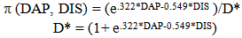 | (6) |
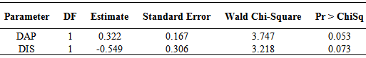
Where (DAP, DIS) is the estimated probability that the team of interest will win the game with difference in average points, DAP, and difference in seeds, DIS, in model.Table 3.5. Logistic Regression Model Parameter Estimates
 |
| |
|
The logistic model was found to be appropriate by the Hosmer and Lemeshow Goodness of Fit test.
3.4. Validating the Models Using Round-By Round Results in 2013
The three point spread models were used to estimate the point spread round by round for each game in the 2013 tournament in an effort to try to predict which team will win the game. Tables 3.6-3.8 summarize the results with the results for Round 3 through the championship game summarized in Table 3.8. Table 3.6. Accuracy of Least Squares Regression Model when predicting first round of 2013
 |
| |
|
Table 3.7. Accuracy of Least Squares Regression Model when predicting second round of 2013
 |
| |
|
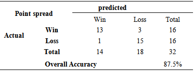
Table 3.8. Accuracy of Least Squares Regression Model when predicting third and higher rounds of 2013
 |
| |
|
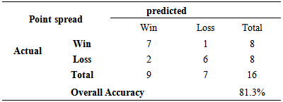
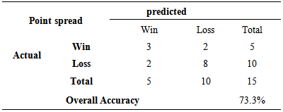
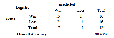
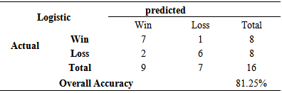
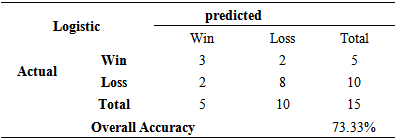
The three logistic models were used round by round to determine which of two teams would win the game for each game in a round. The predicted results were compared with the actual results and the overall accuracy for each round with results from rounds 3-6 combined together are given in Tables 3.9-3.11.Table 3.9. Accuracy of Logistic Regression Model when predicting first round of 2013
 |
| |
|
Table 3.10. Accuracy of Logistic Regression Model when predicting Second round of 2013
 |
| |
|
Table 3.11. Accuracy of Logistic Regression Model when predicting third and higher rounds of 2013
 |
| |
|
The accuracy of the least squares regression models compared with the logistic regression models are very close.
3.5. Bracketing the 2014 Tournament before Tournament Begins
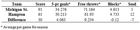
Since the accuracies of the least squares regression models and logistic regression models were very close for the 2013 tournament, we decided to use only the set of least squares regression models to form our bracket for 2014 and predict winners of each round and the overall champion. We applied our first round point spread model to the 32 games in the first round that would be played by the given 64 teams. The model estimated the point spread in the order of points obtained by Team A minus points obtained by Team B. If this model gave a positive result, Team A was predicted to win. It the model gave a negative result, Team B was predicted to win. The model was applied to all 32 games in the first round. Examples from two games in the first round are given to show how the first round model works. The first game considered was between Michigan State and Hampton. Values of the seasonal variables needed for each team for model 1 are given in Table 3.12.Table 3.12. Michigan St. and Hampton Statistics
 |
| |
|
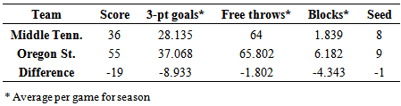
Using the model estimating point spread for games in round 1 (1) in order of Michigan State minus Hampton,  = 1.123*(4.063) - 0.447*(9.234) + 2.295*(-0.12) - 1.684*(-7) = 11.95Since the estimated point spread is positive, the model is predicting Michigan State to win the game. Michigan State did win the game with a final score of 91 to 61.Middle Tennessee and Oregon State also played each other in the first round. Values of the seasonal variables needed for (1) for each of these teams are given in Table 3.13.
Table 3.13. Middle Tenn. and Oregon St. Statistics
 |
| |
|
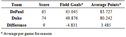
 = 1.123*(-8.933) - 0.447*(-1.802) + 2.295*(-4.343) - 1.684*(-1) = -17.80The point spread was estimated in the order of Middle Tennessee minus Oregon State and since the estimated point spread is negative, Oregon State is predicted to win the game. The actual final score of the game was 36 to 55 with Oregon State winning. The model correctly predicted the winner of 26 games in round 1 and incorrectly predicted the winner of 6 games. The round 2 model given in (3) was used for all the 16 games in this round using the teams predicted by the model in (1) to play each other in this round. As to how this model was used in round 2, an example estimating the point spread of one game in this round will be given. Two teams that were predicted to play each other in this round were DePaul and Duke. The values of the variables needed for both teams to use in the round 2 model (3) are given in Table 3.14.
Table 3.14. DePaul and Duke Statistics
 |
| |
|
Using the model given in (3), the predicted point spread in the order of DePaul minus Duke was given by the following Since the point spread was estimated to be negative, it was predicted that Duke would win the game. This model incorrectly predicted a loss for DePaul who won the game with a score of 74 to 35. For round 2, the model correctly predicted 9 games and incorrectly predicted 7 games.Games played in rounds 3-6 of the tournament used the model developed in (5). An example of a game predicted in round 3 was between South Carolina and North Carolina, two teams predicted to play each other based on the results from previous models, using the values of variables given in Table 3.15.
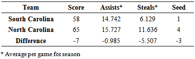
Table 3.15. South Carolina and North Carolina Statistics
 |
| |
|
Estimating the point spread in the order of South Carolina minus North Carolina gives the following result. Since the estimated point spread was negative, it was predicted that North Carolina would win the game. The final score of the game was 58 to 65 with North Carolina winning. The model correctly predicted 6 games in round 3 and incorrectly predicted 2 games in round 3. The model was then used for all predicted games in round 4. The model went on to correctly predict all four games in round 4, both of the games in round 5, and the championship game. One game in round 5 was between Maryland and Notre Dame (which the model had predicted). In order to show further show how this model works (5), the seasonal statistics for Maryland and Notre Dame are given in Table 3.16.
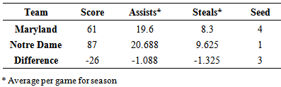
Table 3.16. Maryland and Notre Dame Statistics
 |
| |
|
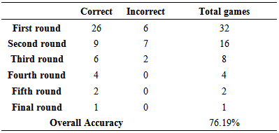
 The point spread is predicted in the order Maryland minus Notre Dame and since this is negative, the model predicted Maryland to lose the game. The final score of the game was 61 to 87 with Maryland losing.The prediction accuracies for each round in 2014 are summed up in Table 3.17.
Table 3.17. Prediction Results of each round for 2014: (Least squares regression model)
 |
| |
|
4. Conclusions
Models were developed to try and explain the point spread between two women’s basketball teams playing in the first round, second round, or third through final rounds of the NCAA women’s basketball tournament. The models were developed using seasonal averages of teams for eight variables in addition to the seed values of the teams. Three variables based on seasonal averages for the teams plus the seed numbers were found to be significant for the model developed explaining point spread of games in the first round of the NCAA tournament. The R-square and adjusted R-square values for the first round model were 0.762 and 0.746, respectively indicating that approximately 75% to 76% of the variation in point spread of the games in the first round is explained by this model. Two variables based on seasonal averages of basketball teams playing in the second round were found to be significant in explaining point spread. The seed number was not found to be significant in this model. The model had R-square and adjusted R-square values of 0.558 and 0.529, respectively indicated that approximately 53% to 56% of the variation in point spread of round 2 games was explained by this model. Two variables based on seasonal averages of basketball teams playing in the third through final rounds of the NCAA tournament plus the seed of the team was found to be significant in the model developed for explaining the point spread for games in the third through final rounds of the NCAA women’s basketball tournament. The models had an R-square and adjusted R-square value of 0.677 and 0.641, respectively. This model explains approximately 64% to 68% of the variation in point spread of games played in the 3rd through final rounds of the NCAA women’s basketball tournament. The three point spread models were tested round by round using data from the 2013 NCAA women’s basketball tournament. The models were tested based on whether or not they could accurately predict the winner of each game, not on how accurately they could predict the actual point spread of each game. The first round model accurately predicted the winner of 28 of the 32 games played in the first round of the tournament in 2013, or the model predicted the correct winner 87.5% of the time. The second round model accurately predicted the winner for 13 of the 16 games, or 81.5% of the time. The third through final round model accurately predicted the winner in 11 of the 15 games, or 73.3% of the games, played in the 3rd through final rounds of the 2013 NCAA women’s basketball tournament.Three logistic regression models were also developed for Round 1, Round 2, and Rounds 3-6 of the NCAA women’s basketball tournament based on data taken from the 2011 and 2012 NCAA tournaments. The HL test was conducted for each of the three models and it was found that there was not sufficient evidence to determine the logistic fit was not appropriate. One variable based on the seasonal average of a team plus the seed value was found to be significant in the first round model. The second round model found only one variable based on the seasonal average of a team to be significant and the third through final round model found only the seed and one other variable based on the seasonal average of a team to be significant. The first round model was used based on data from the first round of the 2013 NCAA tournament and it was determined that the model correctly predicted 29 out of the 32 games correctly (90.63%) as to which team would win the game. A team was predicted to win the game based on this model if the model determined the estimated probability of the team winning the game was greater than 0.50. The model for the second round had a prediction accuracy of 81.3%., and for the third through sixth rounds, the model had an accuracy of 73.3%. In 2014, a continuous process was used to fill in the entire 2014 bracket using the set of point spread models. For this bracket, 76.19% of the games were correctly predicted. In this case, the Round 1 model started with the teams actually playing each other and predicted winners of the 32 games. The average seasonal statistics of the significant variables of the predicted winners of the games in Round 1 were placed into the model for Round 2 and winners for Round 2 were predicted. Seasonal average statistics for these teams were placed into the Round 3 model and winners predicted for Round 3. This process continued to the Final Round and a prediction was made as to who would win the tournament. This prediction was made before any games were played. The number of correct predictions for each round is given in Table 3.17. Out of the 63 games played, the models correctly predicted the winning team for 48 of the games and this is before any games had started. The set of models did a very good job overall and were able to correctly predict the final four, the final two and the winner of the championship.
References
| [1] | NCAA website, last referenced in May, 2014. http://www.ncaa.com/sports/womens-basketball |
| [2] | Carlin, B.P., 1996. Improved NCAA Basketball Tournament Modeling via Point Spread and Team Strength Information. The American Statistician 50: 39-43. |
| [3] | Schertman, N.C., Schenk, K.L., and Holdbrook, B.C., 1996. More Probability Models for the NCAA Regional Basketball Tournaments. The American Statistician, 50: 34-38. |
| [4] | Smith, T., and Schwertman, N.C., 1999. Can the NCAA Basketball Tournament Seeding be Used to Predict Margin of Victory?, The American Statistician, 53: 94-98. |
| [5] | Caudill, S.B., 2003. Predicting Discrete Outcomes with the Maximum Score Estimator: the Case of the NCAA Men’s Basketball Tournament, International Journal of Forecasting 19:313-317. |
| [6] | Kubatko, J., Oliver, D., Pelton, K., and Rosenbaum, D.T., 2007. A Starting Point for Analyzing Basketball Statistics, Journal of Quantitative Analysis in Sports 53:94-98. |
| [7] | West, B.T., 2006. A Simple and Flexible Rating Method for Predicting Success in the NCAA Basketball Tournament, Journal of Quantitative Analysis in Sports, 2(3):3-8. |
| [8] | Zhang, X., 2013. Bracketing NCAA Men’s Division I Basketball Tournament. Unpublished Master’s Thesis Paper, Department of Statistics, North Dakota State University. |
| [9] | Magel, R. and Unruh, S., 2013. Determining Factors Influencing the Outcome of College Basketball Games. Open Journal of Statistics (http://www.scirp.org/journal/ojs). |
| [10] | Kane, M.J., 1996. Media coverage of the post Title IX female athletes: A feminist analysis of sport, gender, and power. Duke Journal of Gender Law & Public Policy 3(1):95-127. |
| [11] | Duncan, M.C., 2006. Gender warriors in sport: Women and the media, A.A. Raney & J. Bryant (Eds.) of Handbook of sports and media, Lawrence Erlbaum Associates, Mahwa, NJ. |
| [12] | Abraham, B., and Ledolter, J., 2006. Introduction to Regression Modeling, 1st ed., Belmont CA: Thomson Brooks/Cole. |
 Abstract
 Reference
 Full-Text PDF
 Full-text HTML