1. Introduction

Location information plays a critical role in wireless sensor networks (WSN). Most of the WSN applications and techniques require that the positions of the sensor nodes be determined. Localisation algorithms (e.g.[1-5]) follow several approaches to estimate positions of sensor nodes.

One approach is to use special nodes, called beacons, which know their own location, e.g. through a GPS receiver or manual configuration. The other nodes that do not know their location, sometimes referred to as unknowns, use different techniques to compute their own position based on the location information of the beacons and the measured distance to these beacons. Once the unknown obtains its position, it could act as a reference for other unknowns.

WSN Testbeds[6],[7] have been used to study various aspects of WSNs. However, the practical difficulties of setting up a WSN and analysing its performance have made simulation essential for the study of WSNs. Simulation is widely used in system modelling for applications ranging from engineering research, business analysis, manufacturing planning and biological science experimentation[8]. There are several simulation packages that can be used to simulate a WSN, such as ns-2[9], OMNET++[10] and TOSSIM[11]. ns-2 is an open-source event-driven simulator designed specifically for research in networks. ns-2 was developed in C++ and uses Object-oriented Tool command Language (OTcl) as a configuration and script interface (i.e., a front-end). Each language has two types of classes. The first type includes the standalone C++ and OTcl classes that are not linked together. The second type includes classes which are linked between the two languages. These C++ and OTcl classes are respectively called, “compiled hierarchy” and “interpreted hierarchy”. These two hierarchies are linked together using an OTcl/C++ interface called TclCL[12].

ns-2 provides substantial support for simulation of TCP, routing, and multicast protocols over wired and wireless networks. Recently, Morávek[13] investigated the capabilities of ns-2 with regards to its suitability to model localisation in wireless networks. This investigation concluded that: ns-2 has all the basic properties to support simulations of different localisation techniques (such as time of arrival (ToA) and received signal strength (RSS)) that are contained in several ns-2 tools and modules; and, ns-2 allowed researchers a high level of independence from the designed framework of the simulator thus allowing developers to modify existing modules or create new modules.

This freedom in ns-2 development, however, means a developer is faced with a large number of implementation options; these require widespread modification of modules and an in-depth knowledge of the inner workings of ns-2.

In this paper, ns-2 is extended to simulate localisation systems in WSNs (Section 3). This extension collects together and leverages existing properties of ns-2 for localisation modelling, offering a simplified and clearly defined development route for implementing new schemes. New modules are added and a base class, called “Position”, is created. Position enables the sensor nodes to estimate their position using the general multilateration method. New classes derived from Position can be created to implement other localisation algorithms as explained in Section 4. A simulation is conducted in Section 5 to evaluate the performance of Position. Results are presented for five localisation algorithms (which are derived from Position) in terms of localisation error, number of references used, remaining energy and distance-measurement error.

2. Localisation Systems

Localisation systems consist of three major components: distance/angle estimation, position computation and a localisation algorithm[14], as shown in Figure 1.

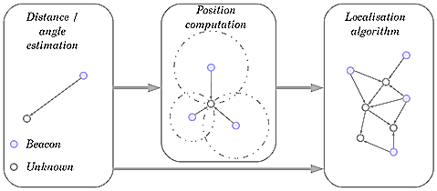Figure 1. Components of localisation systems

• Distance/angle estimation: This component is responsible for determining the physical relationship between two nodes, which can later be used to compute a node's location. Different techniques can be used for this purpose, such as RSS, ToA, time difference of arrival, angle of arrival or round-trip time. These techniques have been investigated in more detail in[15].

• Position computation: This component is responsible for computing the position of a node based on available information about the distance estimated from the previous component and position of references. Recognised techniques used in this component include triangulation[3], trilateration[16] and multilateration[17].

• Localisation algorithm: This is the main component of a localisation system. It determines how the available information will be manipulated in order to enable most or all of the nodes of the WSN to estimate their position.

In the extended ns-2, the RSS technique is used to measure the distance between the node and beacons (or references). The general multilateration method is used in the component for position computations. Following this framework will simplify any future modifications. For example, a new technique (e.g. ToA instead of RSS) can be easily implemented without modifying the entire system.

2.1. Multilateration Method

By using the multilateration method, a node within the range of at least three beacons can estimate its position by minimising the differences between the measured distances and the estimated Euclidean distances in order to obtain the minimum mean square estimate (MMSE) from the noisy distance measurements. As shown in Figure 2, a sensor node has a set of m reachable beacons with the following information (x_j, y_j, d_j), where (x_j, y_j) is the location of beacon j and d_j is the measured distance to it. Assuming that is the estimated position of the sensor node, the error of the measured distance to beacon j can be represented as

(1)

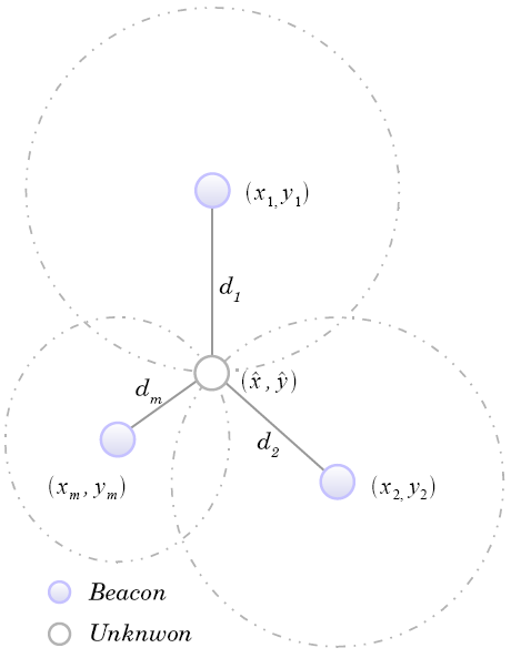Figure 2. Multilateration

This system of equations can be solved to estimate the location by using the matrix solution for MMSE[18] given by:

(2)

where

3. Localisation Extension Structure

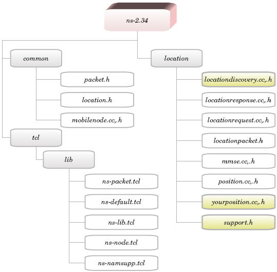
ns-2 contains several flexible modules for energy-constrained wireless ad-hoc networks, which encourages researchers to use ns-2 to investigate the characteristics of WSNs. However, to implement and evaluate localisation algorithms, ns-2 should be extended and new modules should be added. This section describes the class and file structure of the localisation extension presented in this paper. The main purpose of this extension is to provide researchers with a simplified development path when evaluating localisation schemes. Although the entire structure is presented for the sake of completeness, not all the classes and files need to be modified to implement a new scheme. Only the classes and files shaded in yellow in Figure 3, Figure 4 and Figure 5 need to be customised.

Figure 3 shows the new classes that were added to ns-2. These classes can be divided into two types. Firstly, there are standalone classes, which are MMSE, Position and YourPosition classes. These classes are used only from the C++ domain. Secondly, there are compiled hierarchy classes, which are LocDisApp, LocReqAgent and LocResAgent classes. In fact, no OTcl modules were created. However, in order to be able to access the newly compiled hierarchy classes LocDisApp, LocReqAgent and LocResAgent from the OTcl domain, these classes were mapped and linked to corresponding OTcl classes, which are Application/LocDis, Agent/LocReq and Agent/LocRes, respectively. In this way the users are able to create an object of the compiled hierarchy classes from the OTcl domain. For example, the OTcl command “set lreq[new Agent/LocRec]” will create a new object of class LocReqAgent.

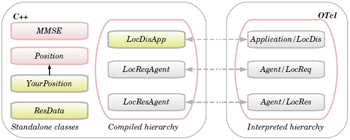Figure 3. The new modules added to the ns-2

3.1. Class Hierarchy

The Doxygen documentation system[19] was used to illustrate the class hierarchy of the new classes as shown in Figure 4. For the sake of simplicity, only the new classes, the classes they are derived from (i.e. parent classes) and the classes used by these new classes were included. Solid lines show where a class is inheriting from another class, for example A → B means class A is derived from class B. Dotted lines show where a class is using a method and/or member of another class.

3.1.1. MMSE Class

This class is responsible for all the mathematical matrices operations required to solve (2). Instead of using general matrix multiplication and matrix inverse, optimized methods dedicated mainly to MMSE were implemented. These optimized methods require less computation and shorter execution time.

3.1.2. Position Class

Position class represents a general localisation method using the basic multilateration method, which was explained in Section 2.1, for position computation and RSS for distance estimation. This method uses all of the available references, does not distinguish between beacons and references, does not weigh the references used and performs the estimation only once. This class is the base class for any localisation algorithms implemented, represented in the text and figures as the YourPosition class. For the sake of simplicity, Figure 3, Figure 4 and Figure 5 include only these two classes, even though other localisation algorithms were also implemented that will be mentioned later.

One of the important methods of this class is “measure_distance_RSS(double Pr);”. This function uses Friis free space equation (3) to estimate the measured distance between the node and the reference (or beacon) nodes,

(3)

where: P_R is the received power, P_T is the transmitted power, G_T is the transmitter antenna gain, G_R is the receiver antenna gain, d is the distance between the transmitter and the receiver, L is the system loss and λ is the wavelength.

To implement a new technique instead of RSS, e.g. ToA, this function should be replaced with a new one. However, this replacement will not affect the other two components, position computation and localisation algorithm, of the localisation system.

3.1.3. YourPosition Class

This class is derived from Position class and is the core class for defining a new localisation scheme. Compared with the Position class, the YourPosition class will include functions specific to the scheme being implemented. For example, for an implementation of ALWadHA[1], one of the schemes tested in Section 5, this class would include scheme-specific methods, such as the smart reference-selection method specified number of references and termination criterion.

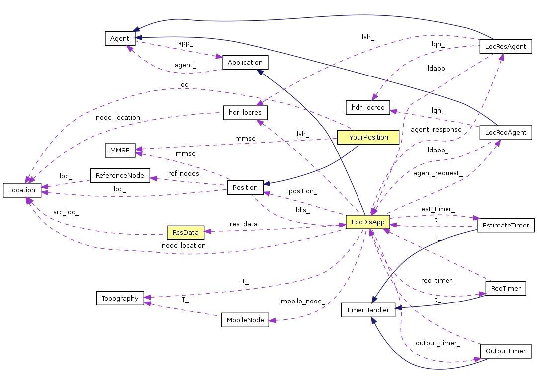Figure 4. Collaboration diagram for the new classes

As shown in Figure 4, the Position class uses the MMSE and LocDisApp classes and the ReferenceNode structure, which consists of two members, location variable and double variable to store the measured distance. The Position class uses an array of this structure (ref_nodes_) to store the location information (location and distance) of neighbouring references. The Location class represents the X, Y and Z coordination of sensor nodes.

3.1.4. LocReqAgent and LocResAgent Classes

These classes are derived from the Agent class. LocReqAgent constructs and broadcasts a “location request” packet. This agent should be attached only to unknown nodes because beacons already know their location. LocResAgent is responsible for handling the packets received. This agent should be attached to all nodes (unknowns and beacons). Two types of packets could be received. The first is a “location request” packet. If this type of packet is received by a beacon or reference node it constructs a “location response” packet that includes location information and then sends it to the requesting node. Unknown nodes receiving this type of packet simply deallocate it. The second is a “location response” packet. The requesting node that receives this packet sends it to the application layer (LocDisApp), which processes the included location information to estimate the node's position.

Two new types of packets were created: firstly, “location request” packet (PT_LOCREQ), which uses the new protocol-specific header (PSH) defined in the structure hdr_locreq; and secondly, “location response” packet (PT_LOCRES), which uses the new PSH defined in the structure hdr_locres. LocReqAgent uses only hdr_locreq to construct “location request” packets. LocResAgent uses both of the headers' structure: it uses hdr_locreq to gain access to, and to process, the received “location request” packets; while it uses the hdr_locres to construct the “location response” packets.

3.1.5. LocDisApp Class

The LocDisApp class is derived from the Application class. Each node in the network uses an object from this class by attaching it to its agent(s). The LocDisApp class performs several functions, such as invoking the broadcast method of LocReqAgent periodically to broadcast a “location request” packet, processing the received “location response” packet and estimating the node location. As shown in Figure 4, this class collaborates with several classes, which are the three timers, the two agents, Location and Position classes. It uses the hdr_locres header structure to gain access to the received “location response” packets in order to process the included location information and estimate the node location. LocDisApp uses a vector of class ResData, which is used to store the location information received from neighbouring references.

3.1.6. The Timer Classes

Three timer classes were created, which are the ReqTimer, EstimateTimer and OutputTimer classes. These classes are derived from the TimerHandler class. These timer classes collaborate with LocDisApp to schedule several tasks during the run time. The ReqTimer is used to moderate how frequently sensor nodes broadcast a “location request” packet. After sending the “location request” packet, the EstimateTimer is used to schedule the estimation process after a specific delay, which is required to give “location response” packets enough time to receive information from neighbouring references. The OutputTimer is used to schedule the action of recording the result (such as location error, number of references used and remaining energy) to the trace file.

3.1.7. ResData Class

This class is responsible for storing and retrieving the location information included in the “location response” packets received from the neighbouring references. This information includes the address, the location and the power with which the packet is received. Implementing a new localisation algorithm could require adding extra attributes to this class. For example, ALWadHA algorithm[1] introduced the term “probability of accuracy” of the reference nodes, which requires selecting a subset of references that will be used to estimate node's position. Therefore, implementing ALWadHA requires adding a new attribute that represents the “probability of accuracy”, to this class.

3.2. The File Structure of the ns-2 Extension

Figure 5 shows the file structure of the new ns-2, where the files under the “location” directory represent the new files that were added to ns-2, while the other files (left-hand side) are the modified files.

Figure 5. The structure of the new ns-2, showing the new files added to ns-2 (right-hand side) and the modified files (left-hand side)

The new classes that were discussed in the previous section are implemented in the files under the “location” directory. In addition to these new files, some other files were modified as follows:

• common/packet.h: Two packet types were created in the locationpacket.h file using two structures (hdr_locreq and hdr_locres). In order to use these two types of packets, their corresponding packet types (PT_LOCREQ and PT_LOCRES) were defined in the packet.h file.

• common/location.h: This file contains the Location class, which is used to represent the location coordination (X, Y and Z) of nodes. Some methods were added to this class, such as: the getter and the setter of an individual coordinate; is_equal( ) method to check if two locations are the same; and distance( ) method to find the actual distance between two locations.

• common/mobilenode.cc, .h: Two methods were added to these files. The first is to get an object to the topography. The second is to record the result in the trace file. The result could be the location error, number of references used and remaining energy. However, this method can be modified to record other information. For example, to implement a new successive refinement localisation algorithm (e.g.[1],[5]), this method can be modified to record the number of iterations required to reach the final estimation.

• tcl/lib/ns-packet.tcl: In order to activate the new header classes, the OTcl class names were included in this file. The new OTcl header classes are “PacketHeader/LocReq” and “PacketHeader/LocRes”, and so only “LocReq” and “LocRes” were added to the active protocol list.

• tcl/lib/ns-node.tcl: As mentioned before, from the localisation perspective, the node could be a beacon, reference or unknown. In order to specify the type of nodes, a new instvar, called “nodeAttribute_”, and a new instproc to get the node attribute, called “attribute”, were created.

• tcl/lib/ns-lib.tcl: In order to enable the simulator to deal with the node attribute, an instproc was created to set the instvar “attribute_”. Within the “Simulator instproc create-wireless-nodes” the node is allowed to set its attribute ($node set nodeAttribute_ $attribute_).

• tcl/lib/ns-namsupp.tcl: During the simulation, when the unknown nodes estimate their position they change their colour (for instance to red). In order to enable the nodes to change their colour after running the simulator, the “Node instproc color” was modified within this file.

• tcl/lib/ns-default.tcl: Sometimes it is necessary to bind some variables in both hierarchies (i.e. interpreted and compiled hierarchies). The default value of these bind variables is initialised in the ns-default.tcl file. Several variables were bound, such as: the packet size; the request frequency (reqFreq_); the showColor_ variable (to enable showing the colour of the nodes based on their attribute); the distanceError_ variable (to consider distance measurement error); and the method_ variable (to specify which localisation algorithm should be applied).

3.3. Localisation Procedures

The complete procedure of the localisation process is as follows:

• LocDisApp schedules the OutputTimer with a specific delay (e.g. 1.0 s) to record the result into a trace file.

• LocDisApp schedules the ReqTimer with a specific delay, which determines how frequently the node broadcasts a “location request” packet.

• At the expiration time of ReqTimer, the LocDisApp invokes the LocReqAgent's method called broadcast( ) in order to broadcast a “location request” packet, schedules the EstimateTimer to start location estimation after a specific delay and reschedules the ReqTimer.

• LocReqAgent constructs a “location request” packet, and then it broadcasts the packet to the neighbouring nodes.

• The LocResAgent of the reference nodes that received the “location request” packet requests the location information of the node from the LocDisApp. LocResAgent constructs a new “location response” packet, which includes this information, and sends it back to the requesting node.

• The LocResAgent of the requesting node receives the “location response” packets from neighbouring references and then sends them to LocDisApp for more processing.

• LocDisApp extracts the required information from the packet received, namely the address and location of the sending reference node and the power with which the packet is received, and then stores this information in a ResData vector.

• At the expiration time of EstimateTimer the LocDisApp invokes the Position's method (or one of its child classes method) called estimate( ).

• Position estimates the node location using the data stored in the ResData vector based on the multilateration method.

3.4. Guidelines for Running the Simulation

Using the ns-2 extension does not require new knowledge or writing a specific code to run the simulator. Normal users who have the basic knowledge to run a simple wireless network using ns-2 are able to write a simple OTcl script to simulate the proposed localisation system. This section gives some guidelines for configuring the localisation simulation. It assumes that the reader is familiar with setting up wireless mobile network simulations in ns-2. Therefore, it will not explain the entire simulation procedures; rather it will show how to configure nodes to simulate localisation. However, the reader is referred to[9] for some tutorials about configuring wireless networks.

At the beginning of the simulation there are only two types of nodes, beacons and unknowns. Each of them has a different configuration, as shown in Figure 6. Beacons already know their location, so they should be attached only with LocResAgent. Unknowns should be attached with LocReqAgent in order to allow them to broadcast location request messages, and they should also be attached with LocResAgent to handle the recipient packets (which are “location request” and “location response” packets). These two types of agents should be attached to LocDisApp.

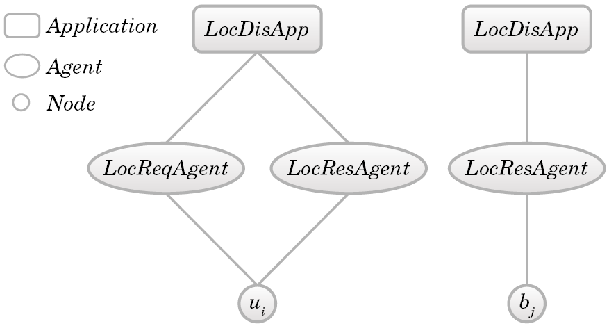Figure 6. Node configuration, where ui is an unknown node and bj is a beacon node

Before creating the nodes their configuration (e.g. the routing protocol, MAC type, etc.) should be specified. In addition, the attribute (either BEACON or UNKNOWN) of the nodes should also be specified; this can be done with the help of the command “node-config”. For example, the following code shows how to create 7 unknown nodes and 3 beacon nodes:

set val(nn) 10 ;# Number of nodes

set val(nu) 7 ;# Number of unknowns

set val(nb) 3 ;# Number of beacons

# Unknown nodes

# Nodes configuration

set val(attr) UNKNOWN ;# node attribute

$ns_ node-config -attribute $val(attr)

# Nodes creation

for {set i 0} {$i < $val(nu)} {incr i} {

set node_($i)[$ns_ node]

}

# Beacon nodes:

set val(attr) BEACON ; # Node attribute

$ns_ node-config -attribute $val(attr)

for {set i $val(nu)} {$i < $val(nn)} {incr i} {

set node_($i)[$ns_ node]

}

The next step is to create the required agents and applications based on the configuration shown in Figure 6.

# unknowns have both request and response agent

for {set i 0} {$i < $val(nu)} {incr i} {

#Setup the request agent

set lreq_($i)[new Agent/LocReq]

$ns_ attach-agent $node_($i) $lreq_($i)

#Setup the response agent

set lres_($i)[new Agent/LocRes]

$ns_ attach-agent $node_($i) $lres_($i)

#Setup the location discovery application

set ldis_($i)[new Application/LocDis]

$ldis_($i) attach-agent $lreq_($i)

$ldis_($i) attach-agent $lres_($i)

}

# Beacon nodes have only response agent

for {set i $val(nu)} {$i < $val(nn)} {incr i} {

# Setup the response agent

set lres_($i)[new Agent/LocRes]

$ns_ attach-agent $node_($i) $lres_($i)

# Setup the location discovery application

set ldis_($i)[new Application/LocDis]

$ldis_($i) attach-agent $lres_($i)

}

Finally, the location discovery applications should be started at a specific time:

# Start the locdis applications

for {set i 0} {$i < $val(nn)} {incr i} {

$ldis_($i) set random_ 1

$ldis_($i) set method_ 2

$ldis_($i) set showColor_ 1

$ldis_($i) set distanceError_ 1

$ns_ at 0.0 "$ldis_($i) start"

}

If required, the user can change the default setting of the bind variables before starting the applications. For instance, in the above code, the random_ variable was set to 1 for all the LocDis applications so that the location request messages could be broadcast at random times instead of starting immediately (random_ = 0). The method_ variable specifies which localisation algorithm should be applied to estimate the node location. The variable showColor_ is used to change the colour of all the unknowns after they estimate their location; setting this variable to zero disables this feature. To consider the distance measurement error, the user should set the distanceError_ variable to 1.

3.5. Manipulate Output Files

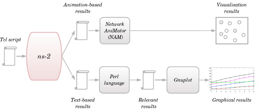
After simulation, ns-2 outputs either text-based or animation-based simulation results. As shown in Figure 7, several tools could be used to interpret these results graphically or interactively. The Network AniMator (NAM)[9] is an animation tool that uses the animation-based results to view the network simulation traces and real-world packet traces. NAM supports topology layout, packet level animation and various data inspection tools.

Figure 7. Tools used to manipulate the result

Text-based results consist of a lot of details on events that occur in the network, such as the sending or receiving of packets, and the movement and remaining energy levels of nodes. A new method was written that records the localisation-related information in the trace file. The format of the traced data is shown in Figure 8. Several tools can be used to extract this location information into a different file, such as the “grep” command. Assuming that the name of the trace file is “location.tr”, then the extracted location information can be store in the file named “result” by using the following command:

grep "^L" location.tr > result

which means: filter only those lines that begin with the letter L.

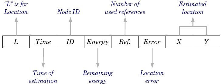Figure 8. The format of the traced location information

To analyse particular data, such as localisation error, the relevant information needs to be extracted from the traces and transformed to a more easily comprehensible format. Perl language[20] was used for this purpose. Perl stands for “Practical Extraction and Report Language”. Perl can be used to filter and to process the ASCII trace files in Unix. For example, a simple Perl script could be written to estimate the average localisation error of all nodes at each second. The Gnuplot software was used to represent the relevant results graphically. Gnuplot[21] is a portable command-line-driven graphing utility for Linux, as well as many other platforms.

4. Implementing New Localisation Algorithms

Implementing new localisation algorithms using the ns-2 extension is a straightforward process. Assuming that one needs to implement a new algorithm called “Your”, then the following procedure should be followed:

1. Create two new files “yourposition.h” and “yourposition.cc” under the “location” directory (see Figure 5), and then modify the ns-2 “Makefile” by adding the corresponding object file name of the new module (-I./location/yourposition.o).

2. Derive a new class called YourPosition from the Position class, and then implement the new methods and features which were not provided by the Position class.

3. In the file “support.h” assign a number for the new algorithm (e.g. #define YOUR 10). If the new algorithm requires extra information for localisation, then this information should be added to the ResData vector within this file.

4. To enable the user to run the new algorithm by specifying the value of the method_ variable to “10” (as explained in Section 3.4) add these few lines to the switch case in “locationdiscovery.cc” file:

switch (method_)

{........

case YOUR:

position_ = new YourPosition(this);

break;

}

5. Finally recompile ns-2.

As an example, let us consider the implementation of the Nearest localisation algorithm which proposed in[3]

1. Create two new files “nearestposition.h” and “nearestposition.cc” under the “location” directory, and then modify the ns-2 “Makefile” by adding the corresponding object file name of the new module (-I./location/nearestposition.o)

2. Derive a new class called NearestPosition from the Position class, and then override the “estimate” method. The new “estimate” method will differ in two things. Firstly, it sets the number of references used to 3 (num_ref_ = 3;) instead of using all the available references. Secondly, it invokes a new method called nearest_ref(). The new method “nearest_ref” will be used to select the closest three references, which will be used in the position estimation.

3. In the file “support.h” add the following:

#defineNEAREST3 2

4. Add these few lines to the switch case in “locationdiscovery.cc” file:

switch (method_)

{........

case NEAREST3:

position_ = new NearestPosition(this);

break;

}

5. Finally recompile ns-2.

5. Simulation Results

To evaluate the effectiveness of the presented ns-2 extension, six localisation algorithms have been implemented for the performance comparison, using the same assumptions. Two algorithms based on the basic multilateration method were implemented. The first one is based on the single-estimation approach (called M_Single), where the node estimates its position only once. The second one is implemented based on the successive refinement approach (called M_Refine), where the node keeps re-estimating its position. The other algorithms are: Nearest[3]; CRLB (Cramer-Rao-Lower-Bound)[4]; NDBL (node distribution-based localisation)[5]; and ALWadHA[1].

Twelve beacons and 64 unknowns were distributed randomly in a 200 m x 200 m field. Several experiments were performed. In each experiment the simulation was run 100 times; the duration of each run was 600 s (the total duration was 60 000 s) and in each run, nodes were redistributed randomly in different places (using a different seed value). RSS was used to measure the distance between nodes. However, to simulate noise (assuming that distanceError_ variable is set to 1), each measured distance was disturbed by a normal random variant with the following settings: a mean of 0.1% of the measured distance and a standard deviation of 1% of the measured distance. The implemented algorithms were evaluated in terms of the location error, number of references used, remaining energy and distance-measurement error.

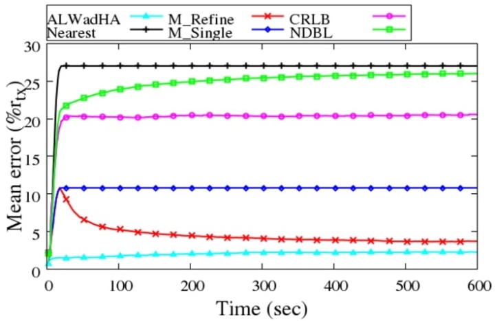
5.1. Localisation Error

The mean error is estimated every second for all knowns as a ratio of transmission range. The mean error at a specific time t is equal to the summation of the location error of all knowns divided by the number of these knowns and then it is divided by the transmission range (r_tx) as follows:

(4)

Where: n is the total number of knowns at a specific time t; z_i is the actual node's location; and is the estimated node's location. Figure 9 shows the mean error of the implemented algorithms.

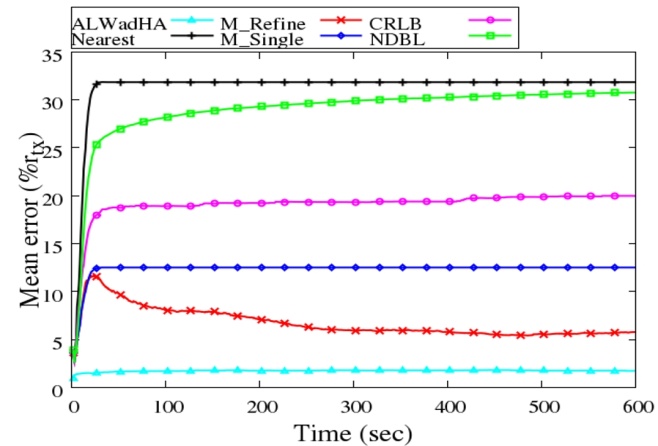Figure 9. Mean error as a ratio of transmission range

5.2. Number of References

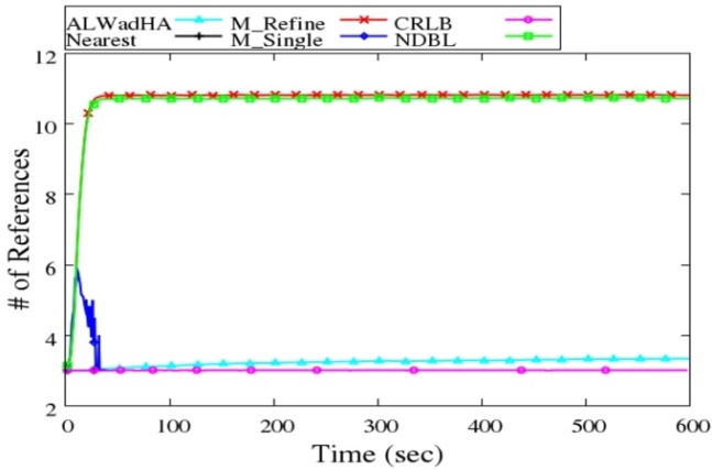Figure 10. Average # of references

Increasing the number of references could enhance the accuracy of the position estimation. On the other hand it increases the complexity of computations. The multilateration method uses all the available references. The number of references used for the Nearest and CRLB algorithms is predefined manually to three references. The ALWadHA and NDBL algorithms specify the number of references dynamically at each iteration, based on a specific criterion. The average number of references used at a specific time t is calculated as follows:

(5)

Where: n is the total number of knowns at a specific time t; S_i is the subset of references used to estimate the location of node i; and C(S_i) is the cardinality of set S_i. Figure 10 shows the average number of references used by each algorithm.

5.3. Remaining Energy

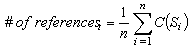
At the beginning of the simulation each node has 2.0 J. Figure 11 shows the average remaining energy versus time considering only energy consumption due to communication.

Figure 11. Remaining energy, j = joule

5.4. Distance-measurement Error

In order to check the robustness of the localisation algorithms with the existence of error, the value of the standard deviation is changed from 1% to 10% of the measured distance. 10 experiments were performed with different standard deviation, and then the mean error was recorded at the end of the run time, as shown in Figure 12.

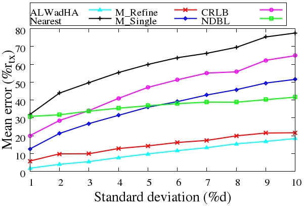Figure 12. Mean error vs standard deviation

5.5. Grid Deployment

In this experiment 12 beacons and 68 unknowns were distributed in a 200 m x 200 m field as a grid. Figure 13 shows the mean error of the implemented algorithms in the grid deployment.

Figure 13. Grid deployment with distance error

6. Conclusions

Academic papers focus on results and rarely include details of how ns-2 simulations are implemented, and if published the modules tend to be scheme-specific. This paper presents an extension to ns-2. The extended ns-2 is a reusable and customisable package that will enable a user with a basic knowledge of ns-2 to simulate a localisation system within a wireless network without any extra knowledge. We showed the simple procedures that are required to implement new localisation algorithms using the extended ns-2. Therefore, the extended ns-2 will eliminate the need to build simulations largely from first principles. This paper will help researchers who want to implement and test new or existing localisation algorithms. Moreover, considering the limited academic publications available, it will also help the new ns-2 users who wish to know more about how a simulation project is built and structured. We also hope that this paper will encourage practitioners in other areas of WSN research to develop similar ns-2 extensions.