-
Paper Information
- Next Paper
- Paper Submission
-
Journal Information
- About This Journal
- Editorial Board
- Current Issue
- Archive
- Author Guidelines
- Contact Us
Science and Technology
p-ISSN: 2163-2669 e-ISSN: 2163-2677
2017; 7(2): 35-40
doi:10.5923/j.scit.20170702.01

Drift Estimation in Offshore Process Measurand
 Abstract
 Reference
 Full-Text PDF
 Full-text HTML
Eze A. U. E, Ossia C. V., Edeh O. D. F.
Offshore Technology Institute, School of Graduate Studies, University of Port Harcourt, Nigeria
Correspondence to: Ossia C. V., Offshore Technology Institute, School of Graduate Studies, University of Port Harcourt, Nigeria.
| Email: |  |
Copyright © 2017 Scientific & Academic Publishing. All Rights Reserved.
This work is licensed under the Creative Commons Attribution International License (CC BY).
http://creativecommons.org/licenses/by/4.0/

The importance of effective measurement of process measurands in offshore oil and gas processing facilities cannot be over emphasized. Due to environmental influences, aging, vibration, wear and tear, etc over-time, these measurement systems experience drifts, giving misleading information about the process variables. In this study it was desired to evaluate the drift in 3 pressure Gauges at an offshore platform. Periodic inspections were performed on the Gauges over a 6-month period. Results showed zero and minor drifts in the measurands after 1-month and 3-monthsusage, respectively. However, after 6-months usage, significant drifts were recorded, corroborating the rule-of-thumb for pressure measurands. The drift models were linear with R2= 1.0 for measurand less than 6 months of instrument usage, and R2< 1.0 for usage periods ≥ 6 months. Recalibration results showed instability for input pressures ≥50% gauge range, and hence faster convergance for input pressures ≤ 50% of gauge range. Validation results showed variance and standard deviation 3685Psi (25.407MPa)and 60.7Psi (0.418MPa), respectively for Gauge 3 at 4000 Psi (27.579MPa)input pressure. To restore the Gauges, recalibrations by error convergence and validations by replications were performed.
Keywords: Measurand, Drift, Deviation, Calibration Error
Cite this paper: Eze A. U. E, Ossia C. V., Edeh O. D. F., Drift Estimation in Offshore Process Measurand, Science and Technology, Vol. 7 No. 2, 2017, pp. 35-40. doi: 10.5923/j.scit.20170702.01.
Article Outline
1. Introduction
- Offshore platforms are located in remote and demanding environment, making oil processing and production not only difficult, but also very risky. For safe and efficient operations, various process instruments (pressure, temperature, level, flow, etc) are installed at designated positions to measure, monitor, control and regulate the operations of the processes within desired operating limits. Over time, harsh environmental impact on these process instruments inevitably results in deviation from set standards and normal operating conditions. This, no doubt, could be very dangerous as it conveys misleading and false information about the process variables. To restore normalcy in process operations, there is therefore the need to determine, validate and recalibrate these instruments periodically. Since calibration tests often require partial or total suspension of production process, estimation of the extent to which an instrument drifts while in service for a specific period becomes paramount. This will ensure that maximum safety, accuracy and efficiency are maintained not only of the personnel, but also of the process equipment and the environment.Complex industrial processes usually involve large number of interrelated physical measurands (pressure, temperature, level, flow, etc). The validity and accuracy of these variables’ sensors determine the safety and reliability of the process. To achieve accurate measurements, instruments that use sensors with high precision and excellent dynamic range/characteristic are used [1].For these sensors validation, Deyst et al [2] summarized the techniques into three groups: Redundant sensor comparison, Limit/Trend checking, and Live zero and ceilings. Although redundant sensor comparison offers fast detection of faulty sensors, it has a number of drawbacks: high cost, sensor noise, transport delay, erroneous detection of fault and common mode failure problems [3, 4]. Limit checking, though useful in detecting gross failure, also are insensitive to subtle degradation of sensors.To get round these challenges, especially with redundant sensor comparison, modern control theory has developed powerful techniques of mathematical modelling, state estimation, and parameter identification. Clark reported the use of model based Analytical Redundancy (AR) [5-8], to validate signals without the use of multiple identical sensors. He pointed out that the more variables that are required to form an analytic measurement, the higher the possibility that large error will propagate into the analytic measurement, causing a higher rate of false alarm. To mitigate for this possible error, Deckert introduced the Least Plant Unit (LPU) [9] which size is smaller when the number of invalidated estimates used in the analytic relationship is minimized. He thus provided a guideline for AR relationship construction which was followed in this study by avoiding the use of invalidated measurements whenever possible.From the deviation and variation in linear and volumetric measurement view point, it is also important to realize that even when all the factors in a measurement process are controlled, repeated observations made during precision measurement of any parameter, even under the same conditions are rarely identical [10]. This is because of inherent variation in any measurement process due to Standard, Workpiece, Instrument, Person & Procedure, and Environment (SWIPE) [11]. This is also known as “Uncertainty in measurement” [10, 12]. However, from Vaisala [13] view point, the key factor about measurement is to understand when it is important to truly know the reliability of measurement results. To this, there are three options: the International System of Units (SI) which says that the farther we are from the SI, the higher uncertainty we have in the measurement in terms of absolute accuracy; Lengthening the calibration interval if the equipment is used with other more stable measurement equipment or if applications grant for the normal calibration interval; shortening the calibration interval when measurement equipment has drifted more than its allowable specification.Calibration requires knowledge of the parameter - measurand, ways of measuring the measurand, and the methods of treating the results. Each one of these will be discussed with focus on measurement of pressure.The calibration process aims to establish the variables that describe the global function of transference of the equipment [14]. So, if the mathematical model that describes this function is linear, the calibration consists of finding the slope and the intercept of the straight line in the graph. Doebelin [15] reported of the static calibration (which curve correlates static input and output variables, and is valuable for the development of functional relation between variables) and dynamic calibration (which correlates the dynamic behaviour of known input and output measurement system). Weather static or dynamic, calibration can still be automated. It only requires a good understanding of the action of each variable in the process and their interrelationship [16]. It also offers automatic documentation and reduction of the procedure cost.In this study, the extent of drift in the process instrument was estimated through periodic calibration with a view to predicting future deviation given similar conditions. Hence, scholars verified the optimal calibration interval; identified the main errors, the primary and secondary elements of pressure sensing; and selected the basic principles and best procedures for calibration. This, in effect, offers not only the required safety, but also quality and profit.
2. Methodology
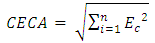
- By ISA standards [17, 18] calibration is a test during which known values of measurand are applied to the transducer and corresponding output readings are recorded under specified conditions. Hence, calibration which was checked at several points throughout the calibration range of the instrument was a comparison of measuring equipment against a standard instrument of higher accuracy to detect, correlate, adjust, rectify, and document the accuracy of the instrument being compared. In this study, statistical tools were used for the drift estimation while deadweight tester was adopted for the calibration of the process pressure Gauge. In doing this, not only was the best practice of ensuring 4:1 accuracy ratio followed [10], but also that the best practice for tolerance and traceability of calibration were adopted. This tolerance should be assigned not only based on the manufacturer’s specification, but also on the requirements of the process, capability of available test equipment and consistency with similar instruments at the facility. Also, calibration should be performed traceable to a nationally or internationally reorganized standard. These were accomplished by ensuring the test standards used were routinely calibrated by “higher level” reference standards.In the oil and gas field, drift in process instruments is absolutely undesirable. The magnitude of this is so much dependent on the amount of use and the length of time it is subjected to the operating environmental hazards. To this effect, uncertainty analysis becomes crucial to evaluate and identify factors associated with the calibration equipment and process instrument that affect the calibration accuracy. Also, of importance is to know how to combine multiple calibration equipment accuracies to arrive at single calibration accuracy. This is shown in Equations (1) and (2).
 | (1) |
 | (2) |
2.1. Periodic Verification
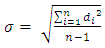
- There were three Cases in this verification process: Case 1 – Verification of the pressure Gauge after 1 month of installation; Case 2 – Verification of the pressure Gauge after 3 months of installation; and Case 3 – Verification of the pressure Gauge after 6 months of installation. With similar instrument features (facial dial, 4-inches), connection (¼-inch MNPT), and conversion (1Bar=14.5Psi), verification tests were conducted on ASHCROFT Pressure Gauges E048025 with Pressure range 0-6000Psi (0 - 14.369MPa), E048020 with Pressure range 0-8600Psi (0 - 59.295MPa), E048029 with Pressure range 0-8000Psi (0 - 55.158MPa) for Case-1 on April 8; Case-2 on July 8, and Case-3 on October 8, respectively. For each Case and each pressure instrument, the input pressure was increased during loading in steps of 25% of the instrument range from 0 Psi, and also decreased back to 0 Psi in the same order for unloading. This was called TPV (True pressure value). For each step increase or decrease, pressure Gauge values were measured thrice. These were termed MPV1, MPV2, and MPV3. Using statistical analyses, estimate of the extent of deviation in the process pressure measuring instrument was made using the standard deviation expression in Equation. (3).
 | (3) |
2.2. Calibration Method
- Deadweight tester, with no matching equipment for pressure calibration in terms of stability, repeatability and accuracy, was the basic primary standard utilized; and its principle has been accepted world over for the most accurate measurement of pressure. It is ideal for calibrating pressure transducers, pressure Gauges, transfer standards, recorders, digital calibrators, etc; and can also be used to measure directly the pressure in system and process where precise measurements are important. The calibration was carried out through the measurement of 5 points uniformly distributed over the calibration range.
2.3. Calibration Procedure
- The American National Standard Institute (ANSI) [12], [13] was the main calibration standard used, and the deadweight principle is based on equation (4):
 | (4) |
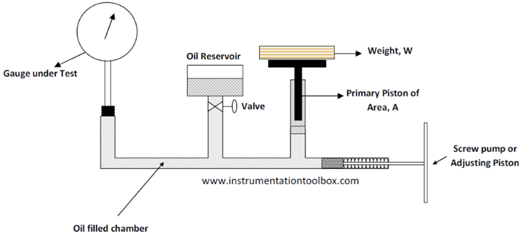 | Figure 1. Setup of Deadweight Tester [19] |
3. Results and Discussion(s)
3.1. Drift Models
- Drift models of the process measurand for the Gauges were observed to be linear within the monitoring period. Two scenarios were considered, namely: (a) Same Gauge with different usage time, and (b) Different Gauges with the same usage time.For Gauge-2, drift model after 6-months was obtained as
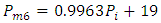 with an associated coefficient of determination R2 = 0.9997 as in Figure 2. However, though not shown in the Figure 2 for clarity, drift model for 3-months was obtained as
 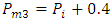 with an associated coefficient of determination R2 = 1. And the drift model for 1-month as
  with an associated coefficient of determination R2 = 1. It can be observed that after 3-replications, the measured pressure value varied linearly with the input (True) pressure; with the slope decreasing from unity with increase in drift. Similar, variation mode was exhibited by Gauge-1, and Gauge-3. The intercept of the models showed the unveiling of incipient zero-error in the instrument as the usage duration increases.Comparing the drift model slopes in Figure 3 with Figure 4, the drift characteristics of Gauge-3 after Month-6 usage can be observed to be higher than that of Gauage-1 within the same usage time. However, the zero error shown as the model intercept can be attributed to environmental effectto which the instrument were exposed.
 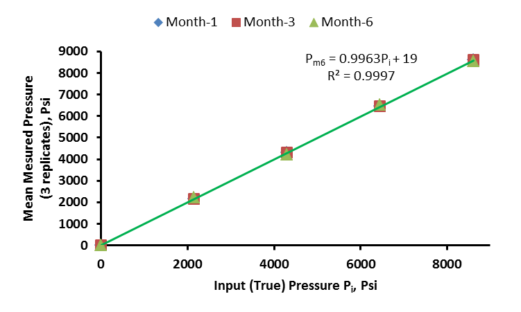 | Figure 2. Drift models for Gauge-2 for Month-1, 3 and 6 usage |
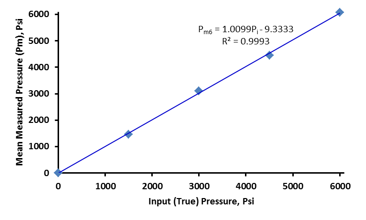 | Figure 3. Drift models for Gauge-1 for 6-Months usage |
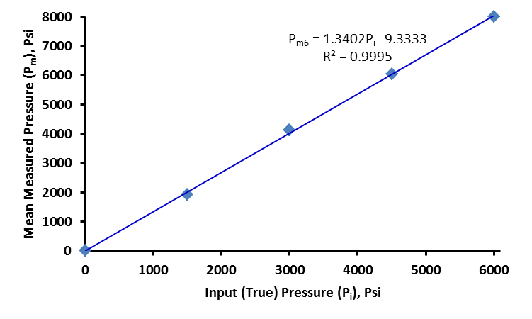 | Figure 4. Drift models for Gauge-3 after Month-6 usage |
3.2. Calibration Results
- In the course of calibration, for Gauge-1, 6-replications (R1, R2, R3, ..., R6) of the operations were performed before the calibration errors were totally eliminated. But for Gauge-2 and Gauge-3, 4-replications (R1, R2, R3, R4) and 5-replications (R1, R2, R3, …, R5), respectively were performed before the calibration errors were completely eliminated.Calibration results for the three pressure Gauges (using different input pressures) are shown in Figure 5, Figure 6 and Figure 7.From the three calibration results, we observe that beyond 50% increase or decrease in the input pressure, the trend was much smoother towards the zero error of the pressure instruments. This suggests that the instruments work at their best below or mid-way their specified pressure ranges. Alternatively, it can be said that it was not recommended to operate the instrument at or close to the maximum specified pressure range, as it has the tendency of more oscillation. These oscillations can be observed in the calibration results at the input pressure curve for 6000Psi(41.369MPa) in Figure 5, 4300Psi(29.647MPa), 6450Psi(44.471MPa) and 8600Psi(59.295MPa) input pressures curves in Figure 6, as well as 4000Psi(27.579MPa), 6000Psi(41.369MPa) and 8000Psi(55.158MPa) inputs Pressure curves in Figure 7.
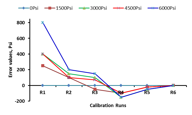 | Figure 5. Calibration results for Gauge-1 at Input Pressures (0 – 6000Psi)(0 – 41.369MPa) |
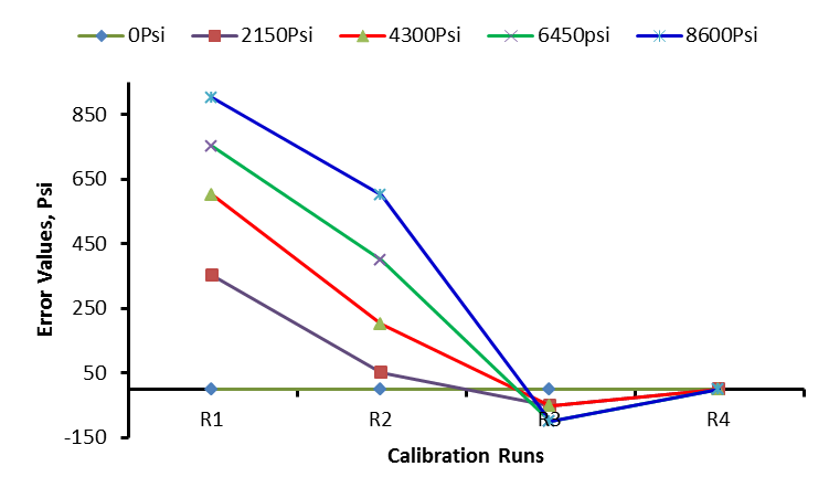 | Figure 6. Calibration results for Gauge-2 at Input Pressures (0 – 8600Psi)(0 – 59.295MPa) |
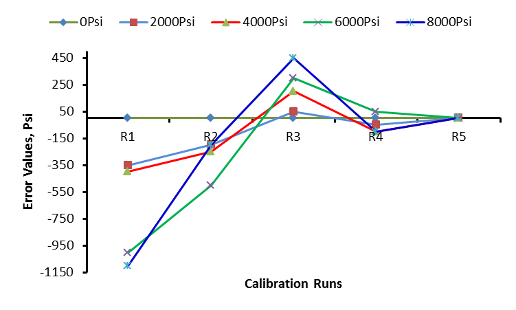 | Figure 7. Calibration results for Gauge-3 at different Input Pressures (0 – 8000Psi)(0 – 59.295MPa) |
3.3. Verification/Validation Results
- It was observed from the verification results that maximum deviation occurred at the 50% (4000 Psi or 27.579MPa) range of Case 3, pressure Gauge-3. Result of this test is shown in Figure 8.
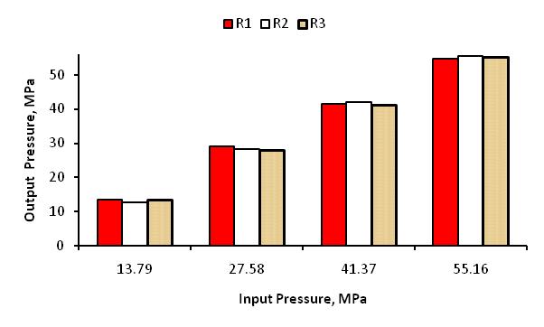 | Figure 8. Test Result for Case-3 which showed maximum deviation |
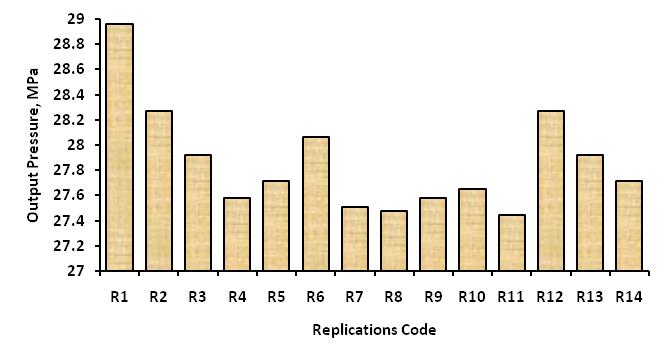 | Figure 9. Output Pressure for Gauge-3 at 4000Psi(27.579MPa) input |
4. Conclusions
- From the three periodic Cases of verification considered for the drift estimation in the pressure process measuring and control instrument, the following conclusions were reached. Firstly, for Case-1, the verification results showed that the pressure Gauges were accurate after one month of installation. In other words, none of the Gauges showed any sign of error due to drift or other factors. The input pressures at any particular range were equal to the output pressures at the same range, implying that the pressures displayed by the instrument were accurate indication of the actual measurand. Hence, there was no need for calibration for any of the Gauges. Plots of the input pressures against the output pressures for the 5 point range considered showed a perfect linearity.Second for Case-2, the verification results showed very slight variation after three months of installation. The variation followed a particular trend for the three Gauges. A maximum variation of 5Psi(0.034MPa) was observed in the Gauge-1 and Gauge-2 with a minimum of 5Psi(0.034MPa) for Gauge-2. This gave a percentage error of 0.0775%. However, this error was insignificant as it lies within the accuracy tolerance for the Gauges (0.1% - 0.5%). A plot of the input pressures against the output pressures for the 5 point range considered showed a perfect linear relationship. This confirms that the variations recorded were insignificant. For this reason, there was no need for Gauge recalibration.Finally, for Case-3, the verification results showed remarkable drifts. A maximum error of 200Psi(1.379MPa) and a minimum of 150Psi(1.034MPa) were recorded on Gauge-3 during the period when the input pressures were 4000Psi(27.579MPa) and 2000Psi(13.790MPa), respectively. This showed a maximum error of 5%, way off the acceptable tolerance. A plot of the input pressures against the output pressures for the three Gauges using the 5 point range considered showed a non-linear relationship. The results also showed that a combination of linearity and span errors contributed to the deviations observed. Hence, the Gauges needed recalibrations to restore the required standards.
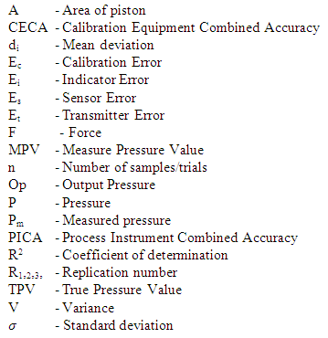
Nomenclature