1. Introduction

Machining is a major process in manufacture used especially to finish mechanical parts. Costs of these operations and final products quality are highly constrained to take into account an increasingly competitive environment, where investors require higher returns on their investments.

Hard machining processes produce high cutting forces and temperatures that affect some cutting process parameters, such as dynamic stability, tool wear, work piece surface integrity, geometrical dimensions. Cutting forces modeling is so necessary, as it permits to characterize material machinability, to get some knowledge on the power required during machining ([1]), to monitor tool wear ([2]), to predict surface roughness and more ([3]). Cutting forces are related to various process parameters ([4]) such as tool material, workpiece properties and cutting conditions (i.e. feed rate, cutting speed, cutting depth,…) ([5]). It is then difficult to provide an accurate theoretical model to describe complex machining processes such as milling and turning.

Artificial neural network (ANN) approach is routinely considered as an accurate and powerful tool for machining process modeling, as it permits to save much time and money generally spent in experimental procedures. A large amount of works have been carried out on forces modeling which have shown that ANN approach is more accurate and faster than many other analytical and numerical cutting force modeling methods. In the working conducted in[6], an approach for cutting forces modeling has been developed, based on feed-forward multi-layer neural networks trained by BP algorithm, and applied to experimental machining data. Szecsi has investigated the effect of two of the main parameters which influence error convergence: learning rate η and momentum term α. While the used analytical model gives an average prediction error of 9.5% on cutting forces, his neural network provides predictions in training with an average error of 3.5%. In[7], Zuperl and Cus have investigated supervised ANN approach to estimate forces generated during end milling process. They have found that the radial basis network requires more neurons than the standard feed forward neural network with BP learning rule and that feed forward neural network gives more accurate results, but takes 70% much time. In milling, using a multi-layer perceptron with BP training method provides a neural network whose error in training is under 2% for all the three force components, and under 4% in testing. As a comparison, an 11% average error is found using analytical methods. In[8], Hao et al. have introduced a cutting force prediction model for self-propelled rotary tool (SPRT). Two types of analyses are presented: simple BP algorithm and hybrid BP algorithm associated with genetic algorithm (GA–BP). Additionally, they have investigated learning rate lr, which controls the adaptation speed of connection weights between neurons, and the momentum rate m, that takes into account the rate of last connection weights changes. A comparison led on the two numerical models shows that GA–BP network predicts SPRT cutting forces more accurately than BP network during training, which is very important for real-time control. Finally, Aykut et al. have tried in[9] to predict cutting forces in asymmetric milling processes using ANNs. Network training has been performed using scaled conjugate gradient (SCG) and feed-forward BP algorithm. Main average percentage errors (APEs) between experimental and numerical Fx, Fy and Fz values have been found around 2% in training and 10% in testing.

Furthermore, some authors have also used opportunities provided by ANN algorithms to predict material behavior in machining: Li et al. has developed in[10] a hybrid model based on an analytical approach using Oxley’s theory combined with a neural network model, in order to predict first cutting forces, temperature in the chip region and chip geometry and then to evaluate workpiece surface roughness, tool wear and chip break ability. They have found errors under 5% on tool wear prediction and 20% on surface roughness and chip breaking ability. Özel and Karpat have compared in[11] exponential regression models and neural network models for tool flank wear and surface roughness predictions during AISI H-13 and AISI 52100 hard turning. As regression models give as good results as ANN models for tool wear prediction, they have found it ineffective to predict surface roughness compared to ANN. At last, Umbrello et al. have developed in[12] a numerical model based on an ANN approach to predict residual stress profile in hard turning of AISI 52100 bearing steel (HRc between 50 and 64). They have especially investigated the optimal number of neurons in the hidden layer and then optimized their model using a hybrid finite element ANN approach ([13]). As a result, their model has given satisfactory results showing a prediction error ranging between 4 and 10%.

In the present study, an ANN approach is proposed to predict cutting force components in hard turning: feed force Fa, radial force Fr and cutting force Ft.

1.1. Experimental Background

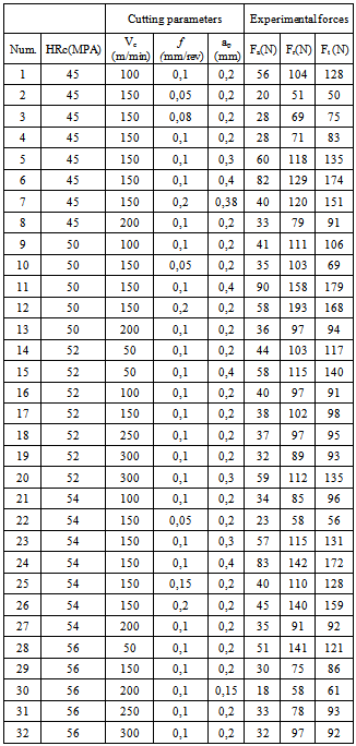
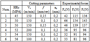
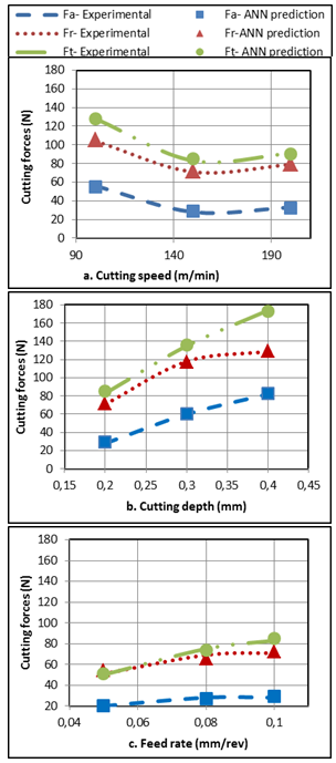
This numerical work is based on a dataset provided by experimental hard turning of AISI 52100 steel using CBN cutting tools ([14]).As shown on Table 1 and 2, three cutting force components have been experimentally determined for 38 different material hardness and cutting condition combinations (cutting speed Vc, feed rate f, cutting depth ap): the first 32 mentioned on Table 1 are used to train the network and the other 6 are testing conditions (Table 2). The main objective is then to develop an ANN model to properly predict cutting condition influence on cutting forces during this hard turning. This model will of course be valuable in the same ranges as training cutting conditions.

Table 1. Experimental training dataset ([14])

Table 2. Experimental testing dataset ([14])

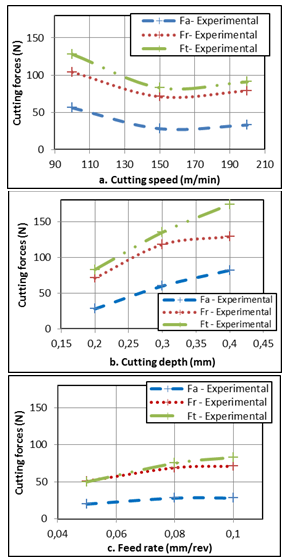Figure 1. Cutting force components as a function of: a.Cutting speed Vc(f=0.1 mm/rev; ap=0.2 mm, 45HRc) b.Cutting depth ap (Vc=150 m/min; f=0,1 mm/rev; 45HRc) c.Feed rate f (Vc=150 m/min; ap=0,2 mm; 45HRc)

As an example, Figure 1 illustrates experimental cutting forces variations with cutting speed, cutting depth, feed rate and workpiece hardness. As mentioned in introduction, many process parameters have a great and complex influence on cutting forces, which can be observed on the provided curves. It is therefore natural to prefer numerical techniques (such as ANN, multiple regressions or genetic algorithm) to analytical modeling to describe efficiently the process complexity.

1.2. Neural Network Modeling

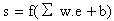
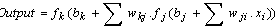
An artificial neural network (Figure 2) consists of simple processors called neurons which are interconnected. This hierarchical network structure has an input layer receiving data e from the outside and an output layer which sends final information to users. In the middle, hidden layers have no direct contact with the environment.

As it has proved its efficiency for approaching non-linear functions ([15]), only BP algorithm has been used for the neural network training. Using notations given on Figure 2, output response is calculated as follow (eq. 1), ([16]):

(1)

During training, weights and biases are initialized to small random values to avoid sharp saturation in activation functions.

Generally, the optimal network configuration is found through statistical error calculation ([17]), between target data c and output data s. The aim is to minimize these errors during training and testing. First, SSE (Sum Squared Error) and SSW (Sum Squared Weights) are evaluated using MATLAB Neural Networks Toolbox. And additionally, two coefficients are calculated to evaluate statistical network performance and reinforce the choice of the best network:

● Linear regression coefficient R (eq. 2).

(2)

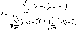
Where Q is the number of cutting conditions, and are mean target and output values.

● Mean absolute percentage error (MAPE) (eq. 3)

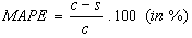(3)

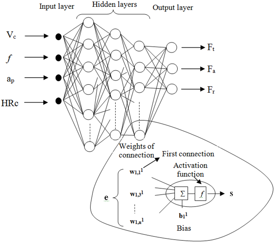Figure 2. ANN Multi-layer feed-forward structure

2. Optimal Choice of an ANN Model

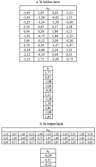
This study is not only focused on its main objective, namely the development of an ANN model to properly predict cutting condition influence on cutting force components. Some major parameters used in the final ANN model have first been optimized:

● The type of activation functions in hidden and output layers

● The number of hidden layers

● The type of training algorithm (Levenberg–Marquardt (LM) or Levenberg–Marquardt using BayesianRegularization (BR/LM) ([18])

● The number of neurons in the hidden layer

In all the following cases, ANNs training are performed on 32 experimental cutting results (Table 1) and their generalization capacities are evaluated on 6 further test data (Table 2), that have of course not been used in training. In each case, input and target values are normalized in the range[-1 -1] to perform an efficient training ([19]).

Two activation functions need first to be chosen: one applied in hidden layers and the second used in output layer to determine on the one hand the appropriate number of hidden neurons and on the other hand output values. Table 3 illustrates results of a preliminary analysis: it gives linear regression coefficients obtained in training (R-training) using two couples of activation functions for a various number of hidden neurons:

● Sigmoid function 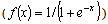in hidden layer and Linear function () in output layer (S.L.)

● Sigmoid function in hidden layer and Sigmoid function in output layer (S.S.)

Table 3. R-training values using S.L. and S.S. activation functions ANN Structure R-Training(S.L.) R-Training(S.S.) 4-4-3 0.952 0,812 4-5-3 0.988 0,805 4-6-3 0.988 0,797 4-7-3 0.993 0,797 4-11-3 0.999 0,785 4-19-3 0.999 0,778 4-24-3 0.999 0,739

It can be noticed that (S.L.) gives more accurate results in each case. This type of activation functions have then been chosen for further study.

Levenberg-Marquardt (LM) optimization algorithm has been used all along this study, in order to find out weights and biases. This training algorithm adjusts them iteratively to reduce error between experimental and predicted output values. It has been shown in literature ([20]) that LM can quickly provide accurate results if the number of neurons in hidden layers is well chosen. Figure 3 illustrates a performance analysis led on this number and based again on R-training values.

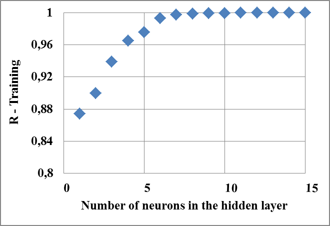Figure 3. R-training variation with the number of hidden neurons (in a single hidden layer configuration)

It can be noticed that using LM algorithm, R-training converges toward a value close to 1 when the number of neurons in the hidden layer reaches 6. However, this algorithm has one major default that should be mentioned: it tends indeed to overfit predicted data in training, which prevents it from accurately generalizing. In this case, the network tends to memorize training examples too well and as a consequence it is not able to give efficient predictions for new cutting conditions. So users need to test their ANN model on a new dataset during the training process, to verify first that the chosen structure gives good results on random cutting conditions and to adjust eventually the structure choice. A solution to improve generalization consists in using Bayesian Regularization, in combination with Levenberg–Marquardt (BR/LM). This algorithm modifies the performance function, which causes the network to have smaller weights and biases and forces the response to be smoother. Moreover, this method is particularly well adapted when the dataset is small.

Figure 4 illustrates MAPE values obtained in testing for a various number of hidden neurons, using an ANN model trained by LM algorithm in black and BR/LM algorithm in grey.

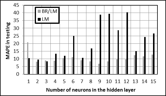Figure 4. MAPE values in testingwith the number of hidden neurons

It can be noticed on Figure 4 that BR/LM gives better MAPEs in testing for all cases when the number of hidden neurons is greater than 7. Moreover, LM algorithm provides very poor results in testing when the number is equal to 9, 10, 11, 12, 14 and 15. This clearly illustrates the overfitting phenomenon mentioned earlier. It is then obvious that Bayesian Regularization should be definitely associated with LM algorithm, as 6 hidden neurons are at least necessary to train correctly the ANN.

Finally, an analysis has been performed to evaluate the value of using two hidden layers instead of one. Various combinations of hidden layers have been investigated in order to build the best network and Figure 5 illustrates representative results provided by a 4-11-3 and a 4-6-8-3 ANN structures (using BR/LM algorithm).

Predicted cutting force components shown on Figure 5 fit experimental values very well in both single and double hidden layers cases. This numerical analysis has shown no advantage in using double hidden layers network.

For further study, a BR/LM training algorithm will consequently be used associated with a single hidden layer and S.L. activation functions.

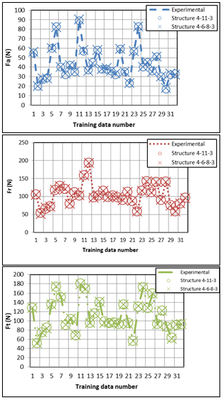Figure 5. Experimental and predicted cutting force components for ANN structures 4-11-3 and 4-6-8-3

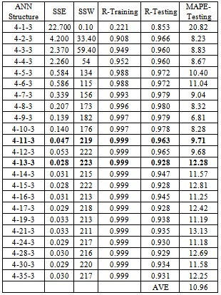
3. Prediction of Cutting Force Components

As explained in introduction, experimental cutting force components have been determined for 38 cutting conditions in which 32 have been used to train the ANN. In order to define the best structure, a various number of neurons in the hidden layer have been tested, from 1 to 35. To evaluate accuracy of the selected structure, cutting force components are calculated for the 6 additional cutting conditions. It can be noticed that testing cutting conditions have to be in the same ranges that the ones used in training.

A key point in the choice of the best ANN structure is the selection of statistical criteria. It is not efficient to limit the study to one criterion. So five representative criteria have been calculated for each structure and representative results have been collected in Table 4:

● SSE and SSW in training

● Linear regression coefficients R in training and testing

● MAPE in testing

Table 4. Statistical criteria values for various ANN structures

SSE as a function of SSW is plotted on Figure 6. A convergence area can be noticed, as the number of neurons in hidden layer reaches 11. As a result, the best structure had to be chosen in this area where SSE is closed to 0 and SSW around 220.

In detail, 4-13-3 structure provides the minimum SSE (0.028) and an optimal R-training of 0.999. But further observations show that this structure doesn’t give the best performance in testing (R-testing=0.928; MAPE-Test = 12.28). It is reasonable to assume that 4-13-3 structure has a little overfitted training data. 4-11-3 and 4-12-3 structures provide accurate predictions in training as well (R-training=0.999), but better results in testing: R-testing=0.963 and MAPE-test=9.71 for the 4-11-3 structure.

So, this analysis leads to select the 4-11-3 ANN structure and the corresponding numerical model has been expressed on equation (4):

(4)

where wji and wkj are respectively the weights that connect input i to hidden layer j and hidden layer j to output layer k, b are biases and f are activation functions.

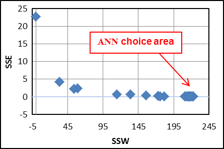Figure 6. SSE and SSW convergence

Weights and biases values are given in Table 5.

Table 5. Statistical criteria values for various ANN structures

Table 6. Experimental and predicted cutting force components in training for the 4-11-3 ANN structure

Experimental and predicted cutting force components are compiled in Table 6. Detailed MAPEs are also given in this Table in order to evaluate the model accuracy.

As expected, this ANN model gives precise results in training: average MAPEs of 1.52%, 0.77% and 1.20% are respectively noted on Fa, Fr and Ft predictions. Figure 7 completes the examples given on Figure 1 with predicted forces. It reinforces the efficiency of ANN predictions in training, as a very good global match is noticed between experimental forces and numerical predictions on all the curves.

Figure 7. Experimental and predicted cutting force components as functions of: a.Cutting speed Vc (f =0.1 mm/rev; ap =0.2 mm, 45HRc) b.Cutting depth ap (Vc=150 m/min; f=0,1 mm/rev; 45HRc) c.Feed rate f (Vc=150 m/min; ap=0,2 mm; 45HRc)

Table 7 illustrates experimental and predicted cutting force components obtained in testing, as well as MAPE values.

Table 7. Experimental and predicted cutting force components in testing for the 4-11-3 ANN structure Experimental forces Predicted forces MAPE Num. Fa(N) Fr(N) Ft(N) Fa(N) Fr(N) Ft(N) Fa(N) Fr(N) Ft(N) 1 42 115 136 27 93 108 35.71 19.13 20.59 2 66 154 143 66 152 139 0.00 1.30 2.80 3 46 139 137 43 135 127 6.52 2.88 7.30 4 36 95 96 39 102 96 8.33 7.37 0.00 5 32 91 94 33 81 89 3.13 10.99 5.32 6 33 81 96 38 103 97 15.15 27.16 1.04 AVE 11.47 11.47 6.17

Average MAPE values of 11.47%, 11.47%, and 6.17% have been respectively found on Fa, Fr and Ft predictions. This ANN model accuracy is similar to what is found in literature ([7]). Figure 8 illustrates finally a graphical comparison between experimental and predicted cutting forces in testing. As shown on Table 7, a good global match is found between numerical and experimental, as 72% of the predicted forces MAPEs are under 11%. However a large discrepancy is noticed on the results, as MAPE ranges from 0 to 36%. Especially, a large error is found with the first set of cutting conditions (HRc=45MPa; Vc=150m/min; f=0.15mm/rev; ap=0.2mm). It seems nevertheless that the ANN model has proven its efficiency, but its accuracy could be further reinforced by optimizing some more ANN parameters, such as learning rate and momentum.

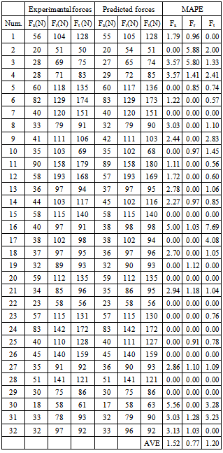
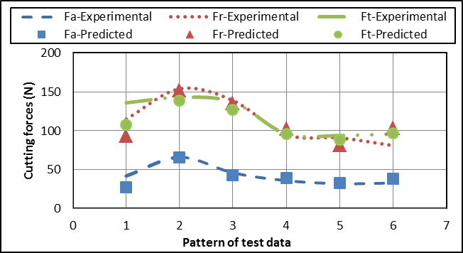Figure 8. Experimental and predicted cutting force components in testing for the 4-11-3 structure

4. Conclusions and Perspectives

The main objective of this study has been to develop a robust numerical model to predict cutting force components in AISI 52100 bearing steel hard turning using CBN cutting tools using an ANN approach.

A precise study has been led to select the more suitable algorithm and methodology:

● The number of hidden layers has been tested. Neither using double hidden layer has shown advantage over single hidden layer.

● The type of transfer functions in hidden and output layers has been investigated. A sigmoid activation function has been chosen in hidden layer and a linear one in output layer.

● Levenberg–Marquardt (LM) algorithm has been compared to Levenberg–Marquardt using Bayesian Regularization (BR/LM). It has appeared that using Bayesian Regularization permits to avoid overfitting in training, which gives thus a major advantage over simple LM algorithm.

● And finally, a various number of neurons in hidden layer have been tested, from 1 to 35. It has been noticed first that the algorithm converges when this number reaches 11, and second that a minor overfitting appears when the number of neurons exceeded 13.

For the selected 4-11-3 ANN structure, which uses BR/LM algorithm, S.L. activation functions and a single hidden layer, an excellent agreement has been found between numerical predictions and experimental data for the 32 cutting conditions used in training (average MAPE under 2%). And a quite large discrepancy has been noted on the 6 tested cutting conditions: MAPE ranges from 0 to 36% on the 18 cutting force components dataset. Globally, the developed ANN model remains nevertheless efficient and as accurate as what is found in literature and should be recommended in machining process modeling.

As a perspective, it seems essential to expand this approach. It could be first possible to compare the proposed numerical approach with analytical models, and then propose hybrid methods based on an analytical approach combined with numerical technics. Moreover, some major ANN parameters such as learning rate and momentum term need to be investigated in order to reinforce the model accuracy. Finally, some other algorithms such as SCG could provide some improvements to the ANN model too.