Kireet Semwal
Department of Physics, GB Pant Engineering College, Pauri (Garhwal), 246194, Uttarakhand
Correspondence to: Kireet Semwal, Department of Physics, GB Pant Engineering College, Pauri (Garhwal), 246194, Uttarakhand.
| Email: |  |
Copyright © 2012 Scientific & Academic Publishing. All Rights Reserved.
Abstract
Snow avalanches are formed in the mountainous snow regions mostly due to the presence of weak layers between the adjacent snow layers. Since the prevailing atmosphere in these regions is stable, weak snow layers are formed due to the presence of surface hoars, which is measured by surface layer heat fluxes. Surface hoar forms when relatively moist air over a cold snow surface becomes over saturated with respect to the snow surface; causing a flux of water vapor, which condenses on the surface, and creates feathery crystals (the icy layer equivalent to dew). Once buried, the resulting weak layer is a serious consideration for avalanche formation. Surface hoar tends to form at night when the snow surface generally cools and the adjacent air becomes over saturated. The surface layer heat fluxes in the atmospheric boundary layer over Himalayan regions are calculated here by stability criteria using the bulk aerodynamic method.
Keywords:
Snow Avalanche, Snow Weak Layers, Surface Layer Heat Fluxes, Surface Hoar, Straitigraphy
Cite this paper: Kireet Semwal, Prediction of Snow Avalanches by Using Surface Layer Heat Fluxes, Science and Technology, Vol. 2 No. 6, 2012, pp. 156-162. doi: 10.5923/j.scit.20120206.03.
1. Introduction
The exchange of heat between the snow surface and the atmosphere is important for avalanche formation. Heat exchange can alter surface snow characteristics and can produce weak snow layers immediately below the snow surface, which may fail or act as a future failure layers after subsequent snowfall. Heat can enter or leave the snow surface by conduction, convection, or radiation. Heat may be transferred to and from the snow surface by turbulent exchange (called sensible heat flux  ). If the air is warmer than the snow surface, heat is added to the snow-pack. If the surface is warmer then the air, heat is lost from the snow surface. Heat may also flow to and from the snow surface by condensation, resulting from the diffusion of water vapour. In this case, the direction of heat flow is from regions of high water vapor concentration to regions of low concentration. Since saturated warm air can hold more water vapour than saturated cold air, the flux of heat (and water vapour), called latent heat flux
  , flows from region of high temperature to low temperature[1]. Hence the magnitude of each energy flux (i.e.
  and
and  ) is influenced by snow surface temperature, the water vapour presence in the air, and the variations in the air temperature and wind speed, i.e. the fluxes depend on turbulent mixing in the first few meter above the snow surface. So the study of these two ambient and snow-surface temperature dependent turbulent fluxes are very important for the prediction of snow avalanche formation. In the present study, we shall calculate these surface layer heat fluxes over a snow surface using mean meteorological parameters in a bulk aerodynamic method.
2. Methodology
The lowest layer of the earth’s atmosphere is called the atmospheric boundary layer (ABL). The boundary layer thickness is quite variable with time and space, ranging from hundreds of meters to two to three kilometers. Transport processes in this boundary layers is in general turbulent; turbulence is therefore the key factor in the vertical exchange of momentum ( ), heat (
 ), and moisture (
 ) between the earth’s surface and the upper atmosphere. Turbulence consists of many different size of eddies superimposed on each other. The size of eddies are of the order of a few millimeters to the depth of the boundary layer. The atmosphere can be stable, unstable or neutral; this stability is measured here by using the Richardson number (
 ). The stable atmosphere is due to the presence of a temperature inversion, and therefore the water vapour content is higher over the snow surface. In the case of an unstable atmosphere, the surface temperature is higher than the upper atmosphere, and therefore the water vapour near the snow surface will move upwards. While in the case of a neutral atmosphere, there is no relative motion of the water vapour.
2.1. Wind Profile
The force exerted on the snow surface by the moving air being dragged over it is called the surface shearing stress (τ) or vertical flux of horizontal momentum. It is the force, which causes the snow particles to move. It is written as:  | (1) |
Or | (2) |
And | (3) |
In integration of equation (2) leads to the well known logarithmic wind profile for the neutral, constant flux surface layer, i.e,  | (4) |
Here the boundary integration constant z0 is the roughness height of the surface (∼ 10-4 m), the level at which the mean wind is presumed to vanishes, i.e, u = 0[2]. The parameters u* and z0 of the given wind profile are obtained from the straight line (4) if the mean wind speed is plotted against ln z. Thus the surface layer stress (momentum flux) may now be calculated by equation (3) as  | (5) |
When the atmosphere is stable or unstable, the similarity theory of Monin-Obukhov[3] suggests that the vertical shear in the surface layer may be represented by the modification of equation (2); i.e’ | (6) |
From equations (1), (5), and (6) we have | (7) |
and similarly according to Casiniere[4] the vertical gradient of potential temperature and humidity in the surface layer have the forms | (8) |
 | (9) |
where ΦM, ΦH, and ΦE are the stability functions (similarity functions). Since the potential temperature removes the temperature variation caused by changes in pressure with height, the potential temperature (θ) is used instead of temperature (T), as | (10) |
Assuming the snow surface is saturated. Using Teten’s formula, that the saturated vapor pressure for boundary layer temperature is defined as [5][6][7][8] | (11) |
and the vapour pressure of the air is[9] | (12) |
Then the specific humidity is defined as[10] | (13) |
2.2. Stability Criteria
According to Cline[11] The Richardson number ( ) is a convenient means of categorizing atmospheric stability (or the state of turbulence) in the lowest layers,
 | (14) |
 relates the relative roles of buoyancy (numerator) to mechanical (denominator) forces, i.e, free to forced convection, in turbulent flow. Thus, in unstable conditions, the free forces dominate; and
  is negative and increases in magnitude with the temperature gradient, but is reduced by an increase in the wind gradient. In a stable (inversion) conditions
  is positive; and in the case of neutral conditions,
  approaches zero. For the stability condition, we use the followings: Stable case: (
 )
)  Neutral case: (
 )
) Unstable case: (
 )
)

2.3. Surface Layer Fluxes
This topic deals with the development of the equations used to estimate the gain or loss of heat by a snow cover; of primary importance is the energy exchange (i.e., sensible and latent heat energy) at the snow-air interface. Under most conditions, the energy exchange at the snow air interface is much greater than the heat transfer at the snow soil interface and depends upon whether it is cold (less than 0℃) or a wet (0℃, often isothermal) pack.The vertical flux of heat due to the internal energy gains or losses by variation of radiation, and heat conduction represented by the convergence or divergence of sensible heat fluxes within the snow pack. The vertical turbulence sensible flux is therefore written in terms of the potential temperature gradient
  and a transfer coefficient
  (m2/s) specifying the effectiveness of the transfer process, known as the eddy difusitivity for heat. It is calculated as
  | (15) |
the transfer coefficient varies with height over the surface and with the condition of turbulence[11]. The direction of the heat transfer (sign of
  ) is determined by the sign of the temperature gradient. Here, sensible heat flux toward the snow cover is taken as negative. Therefore the sensible heat flux is calculated as[12]
 | (16) |
From equations (15) and (16), we have: or
or  | (17) |
The exchange of water vapour between the surface and the atmosphere is determined by the humidity, just as the sensible heat flux is largely governed by the temperature in the lowest layer. However, whereas the heat flux is overwhelmingly into the air by day and returned to the surface by night, the evaporative loss is strongest by day but often continues at a reduced rate through the night. Under certain conditions (like stable atmospheric condition), this loss may be halted, and water is returned to the surface as dew on the snow surface[9]. This is the condition for crust or surface hoar formation and becomes a dominant factor for the occurrence of snow avalanche. The vertical flux of water vapour can be treated similarly as equation (16). The positive sign is assigned for evaporation. The amount of heat per unit volume  is replaced by the mass of the water vapour pre unit volume (
 ). The vertical flux (mass flux) of water can be written as:
 | (18) |
Similarly from equations (7) and (15),  is written as:
 | (19) |
If  is the pressure of water vapour in the atmosphere, then
 | (20) |
and for air  | (21) |
From equation (20) and (21), it follows that  Then equation (16) reduces to
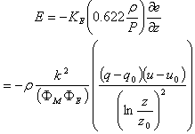 If the surface temperature is
  the pressure of water vapour there is 611 Pa; and if the vapour pressure in the air above the surface is less than this, water from the surface is evaporated. Conversely, if the vapour pressure gradient (air to the surface) is negative, water vapour condenses at the surface, and the surface gains heat at a result. Then the energy required to vaporize the water, i.e., the flux of latent, is given as
 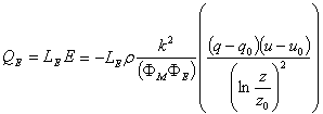 But when the surface temperature is below
  , vapour may sublimate directly over the snow surface as hoarfrost, surface hoar or rime, and then
  is the latent heat released due to the sublimation of vapour over the surface at the rate
 . Avalanches occur when new snow falls over the weak snow layer formed by this condition[13].
3. Study Site and Data Collection
the study site, Patsio (32015´ N, 77027´ E; 3800 m a.s.l), was surrounded by high mountain ridges (Great Himalayan range), has a south facing gentle slope of about 200 to 750 with uneven terrain and is about 160 km from the hill station Manali on the Manali-Leh axis in the North-West Himalaya. This observatory is equipped for the measurements of snow and meteorological parameters. It is a representative site for the study of seasonal snow cover along the whole axis. Snow cover of the season mostly starts by the middle of November and melts off by the middle of May. The mean standing snow cover is of the order of 200 cm, and mean air temperature is approximately -5 to -6℃, based on 7 years of observations. Roads to the site are closed during winter (November to April) due to heavy snowfall resulting from eastward synoptic scale weather systems, such as westerly disturbances.This study was carried out from December to April 1998-99. The parameters used here for the measurements of surface layer fluxes are wind speed and direction, temperatures (minimum, maximum, ambient and snow surface), pressure, relative humidity, which were manually observed. Stratigraphy and MTX data are also used. In the MTX, various temperature sensors were placed at 20-cm intervals from the ground through the snowpack to measure the temperature profile. Each day two observations, viz., 0830 IST and 1730 IST, were made. Stratigraphy observations involved by digging a pit and studying the snow layer characteristics to determine crystal type, hardness, etc. Stratigraphy observations were made once a week between 0730 IST to 0930 IST.
4. Results and Discussion
4.1. Mean Meteorological Parameters
4.1.1. Snow Fall and Standing Snow
During winter 1998-99, the first snowstorm was recorded on 20 December. with 3.0 cm snowfall, and the last snowfall was recorded on 11 April with 2.0 cm snowfall. Also in this season, most snow fall between January and March. The maximum snowfall, 36 cm, was recorded on 23 February 1999.
4.1.2. Temperature
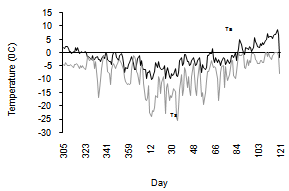 | Figure 1. Variations of Surface & Air Temperatures |
The highest maximum temperature was 12.5℃ recorded on 29 April, and the lowest maximum temperature was -0.6℃ recorded on 2 February. The highest minimum temperature was -0.1℃ on 30 April, and the lowest minimum temperature was -19.5℃ on 1 March. The highest air temperature was 8.8℃ on 30 April, the lowest was -14.4℃ on 16 January, and the average air temperature was -3.3℃.Figure-1 shows that the air temperature was below 0℃ in the evolution period (up to 28 March), and there after it increases above 0℃. The surface temperature was below 0℃ during the whole season (Figure-1). The highest, lowest and average surface temperatures were 0℃ on 28 April, -23.0℃ on 19 January, and -3.4 ℃, respectively.
4.1.3. Wind Speed
Wind speed and direction in the mountains are crucial factors for avalanche formation. The characteristics of wind velocity change with both altitude and the topographic features. Snowfall is generally greater on the windward side (i.e., lifting occurs) than on the leeward side (i.e., subsidence occurs), and therefore the wind velocity causes snow deposition and redistribution. In fact, redistribution of snow can account for avalanche release due to the loading, even in clear weather. The critical (threshold) wind speed at which snow is picked up from the surface by turbulent eddies is a complicated function of snow surface characteristics. Threshold wind speed increases with increasing temperature, humidity, and density of snow. For loose, unbound snow, the typical threshold wind speed (at 10 m height) is 5 m/s. For a dense, bounded snow cover, a wind speed greater than 25 m/s is often necessary for snow blowing. Blowing snow also occurs with modest winds whenever snow is falling. The wind speed was mostly less than 5 m/s during this winter season (Figure-2); therefore, conditions were relatively calm. During winter 98-99 the maximum wind speed was 7.4 m/s on 18 March, the minimum 0.4 m/s on 29 January and average wind speed was 2.0 m/s.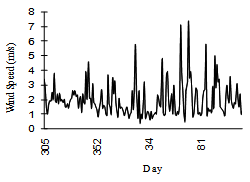 | Figure 2. Variation of Wind Speed |
4.1.4. Pressure
The variations in pressure in the Himalayan regions are due to the westerly disturbances. During winter 98-99, the pressure varied between 635 to 652 mb (Figure-3). The maximum pressure was 651.5 mb on 1 & 3 November and the average pressure during the whole season was 644.2 mb. The minimum pressures were 635 mb on 8 January, 635 mb on 28 January and 636 mb on 1 February, and shows the snowfalls of 17 cm, 34 cm, and 14, cm respectively.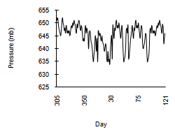 | Figure 3. Variation of Air Pressure |
4.1.5. Humidity
 | Figure 4. Variation of RH% |
 | Figure 5. Variation of Specific Humidity Gradient |
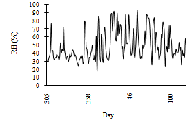
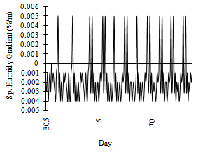
The relative humidity shows that the snow cover is either dry or wet. During winter 98-99, relative humidity varied between 20 and 95%; the maximum, minimum, and average values were 91.5% on 27 January, 24.5% on 3 April, and 54.9% on 9 April respectively (Figure-4). The specific humidity gradient (Figure-5) shows the mass (or vapour) transfer toward or outward from the surface and is calculated from relative humidity and air and surface temperature. There was a very small diurnal specific humidity gradient in the northwest Himalayan regions during the winter 98-99. The mass flow was mostly toward the snow surface during the evolution period (up to 3 March), and thereafter it was outward from the surface. Although the mass transformation is very small, but it is significant for weak-layer (i.e. hoarfrost, surface hoar or rime) formation.
4.2. Derived Parameters
4.2.1. Richardson Number
The Richardson number is calculated here by using the mean values of wind and air temperature (Figure-6). During winter 98-99, the maximum value of  was 2.93 on 15 March, and the average value was 0.5, which is suitable for the “no convection” condition according to Webb (1970) and Braithwaite (1995). During winter 98-99,
  was almost positive during this whole season, and the stable stratification prevailed. This is the essential condition for the weak-layer formation.
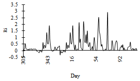 | Figure 6. Variation of Ri |
4.2.2. Sensible heat flux
Since the sensible heat flux shows the amount of heat exchange between the snow surface and the lower atmosphere. The sensible heat flux  was mostly towards the snow surface (Figure-7), which helps the surface snow to melt. Which increase the water vapour near the surface and make the air more saturate then the surface[14].
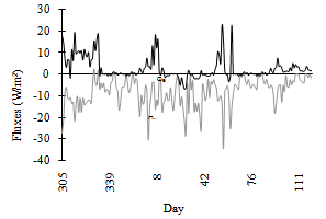 | Figure 7. Variation of Surface Layer Heat Fluxes |
| Table 1. Derived Parameters in Evolution and Depletion period |
| | Derived Parameters | Evolution Period | Depletion Period | | Average Ri | 0.6 | 0.2 | | Average QH (W/m2) | -10.3 | -12.1 | | Average QE (W/m2) | -0.5 | 6.3 |
|
|
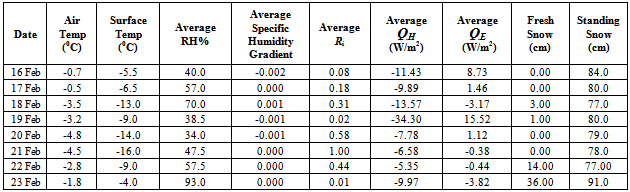
Table 2. Conditions for formation of faceted crystals over the snow surface
 |
| |
|
4.2.3. Latent heat flux
Latent heat flux is the measure of evaporation or condensation of the water vapour at the surface. It depends on the vapour pressure gradient and therefore on the specific humidity gradient and on the wind speed. Since during this season, the air temperature was higher than the surface temperature but less than 0℃ (i.e., both temperatures are negative), the specific humidity gradient was towards the snow surface, the atmosphere was stable, and the wind speed was low (i.e. calm condition). The existence of such conditions is suitable for the formation of surface hoar. The stability of the atmosphere shows that the water vapour near the surface remains near the surface and cannot escape towards the upper atmosphere. The water vapour will condense on the snow surface during any suitable condition of very low temperature (i.e., at night or on cold day). The water vapour ills the pores of the snow surface and condenses around the snow crystals and over the snow surface in the form of a thin, icy layer such as hoar frost, surface hoar or rime. Once such types of weak layers are formed, is a serious condition for avalanches formation, when further snow falls cannot be bound well to the lower snow surface.During the evolution period in the winter 1998-99, condensation occurred up to 18 February 1999, and thereafter evaporation started (Figure-7). The maximum value of  was 22.7 W/m2 on 25 February. and its average value was 3.0 W/m2.
4.2.4. Stratigraphy
The detailed study of the observations of one week (16 February to 23 February 1999) are in Table-2. In this week,  was always towards the surface and air temperature was near the melting point; the crystals formed should be melt-freeze grains. Values of
  show that there was some evaporation on 16, 17, 19, and 20 February, which further condenses over the snow surface and formed surface hoar (facets). The thickness of such types of layers increased due to the condensation with snowfall on 22 and 23 February. Formation of such layers can be verified by snow pit stratigraphy taken on 24 February. This stratigraphy shows that the crystals formed on the uppermost snow layer were faceted, and the snow was dry. The thickness of that layer was of 12 cm. It was found that one avalanche had occurred on 23 February. The reason for this avalanche was the overburden of 36 cm of fresh snow on 23 February over the weak layers formed by the faceted crystals, because the fresh snow cannot bind well to the faceted crystal layers below it.
5. Conclusions
Observations of snow surface turbulent heat fluxes show that when the boundary layer atmosphere is stable, the water vapour near the surface cannot escape into upper atmosphere and remains near the surface. This vapour then condenses over the snow surface when the atmosphere is cold and calm. This condensation process makes a hard icy layer of faceted crystals over the snow surface, which is significant for snow avalanche formation when new heavy snowfall occurs.
NOTATIONS
u Mean wind speed (ms-1) Frictional velocity (ms-1)
 Height of the anemometer (m)
 Surface roughness (∼ 1.7 10-4 m)
 Turbulent shear stress at snow surface (kg m-1 s-2)
 Density of air (kg m-3) i.e.
 Standard density of air (1.29kgm-3)
 Mean atmospheric pressure (mb)
 Standard pressure (∼ 1000 mb)
 Specific heat of air at constant pressure(1005Jkg-1/℃)
 Gas constant
 Von Karman’s constant (∼ 0.40)
 Specific humidity at surface
 Specific humidity at level
 Acceleration due to gravity (ms-2)
 Potential temperature
 Flux temperature scale parameter
 Flux specific humidity scale parameter
 Mean potential temperature
 Diffusion coefficient for viscosity (m2s-1)
 Diffusion coefficient for sensible heat flux (m2s-1)
 Diffusion coefficient for latent heat flux (m2s-1)
 Stability function for momentum
 Stability function for sensible heat
 Stability function for latent heat
 Sensible heat flux (Wm-2)
 Latent heat flux (Wm-2)
 Richardson number
 Latent heat of vaporization or sublimation(2500Jgm-1)
 Molecular weight of air
 Molecular weight of water
References
| [1] | Mc Clung, David and Schaerer, 1993. The avalanche handbook. The Mountaineers Pb. Washington. |
| [2] | Braithwaite, Roger J., 1995. Aerodynamic stability and turbulent sensible-heat flux over a melting ice surface, the Greenland ice sheet. J. Glaciology 44 (139), 562-571. |
| [3] | Monin, A.S., and Obhukhove, A.M., 1954. Basic laws of turbulent mixing in the atmosphere near the ground. Tr. Akad. Nauk SSSR Geophy. 24 (151), 1963-1987. |
| [4] | Casiniere, De La A.C., 1974. Heat exchange over a melting snow surface. J. Glaciology. 13 (67), 55-73. |
| [5] | Stull, R., 1988. An introduction to boundary layer meteorology. Kluwer Press. |
| [6] | Lowe, P.R., 1977. An approximating polynomial for the computation of saturation vapour pressure. J. Appl. Meteor. 16, 100-103. |
| [7] | Bolton, D., 1980. The computation of equivalent potential temperature. Mon. Wea. Rev. 108, 2691-2700. |
| [8] | Buck, A.L., 1981. New equations for computing vapour pressure and enhancement factor. J. Appl. Meteor. 20, 1527-1532. |
| [9] | King, J.C., and P.S. Anderson, 1999. A humidity climatology for Halley, Antarctica, based on frost-point hygrometer measurements. Antarctica Sc. 11 (1), 100-104. |
| [10] | Byer, H.R., 1974. General meteorology. Mc Graw-Hill Pb. |
| [11] | Cline, D.W. 1997. Effect of seasonality of snow accumulation and melt on snow surface energy exchange at a Continental Alpine site. J. Appl. Meteor. 36,32-51. |
| [12] | Panofsky, H.A., and J.A. Dutton, 1984. Atmospheric turbulence: models and methods for engineering applications. New York, etc., John Willy. |
| [13] | Oke, T.R., 1990. Boundary layer climates. Routledge. |
| [14] | Businger, J. A., 1974. A review of flux profile relationships in the atmospheric surface layer. B. L. Meteor. 28, 181-189. |
| [15] | Stakepole, J.D., 1967. Numerical analysis of atmospheric soundings. J. Appl. Meteor. 6, 464-467. |
| [16] | Dyer, A.J., 1974. A review of flux profile relationships. B. L. Meteor. 7, 363-372. |
| [17] | Garratte, J.R., 1992. The atmospheric boundary layer. Cambridge University Press. |
| [18] | Webb, E.K., 1970. Profile relationships: the log linear range, and extensions to strong stability. Q. J. R. Meteor. Soc. 96, 97-90. |
| [19] | Wexler, A., 1976. Vapour pressure formulation for water in range 0 to 100 0C: A revision. J. Res. Nat. Bur. Stand. 80A, 775-785. |
| [20] | G.O. Odhiambo and M.J. Savage, South African Journal of Science 105, May/June 2009, 208-220. |
 Abstract
 Reference
 Full-Text PDF
 Full-text HTML