1. Introduction

Worldwide, efforts are undertaken to reduce carbon emissions in every part of the agrifood supply chain due to growing concerns over global warming and climate change. The escalating levels of carbon emissions have fuelled climate change to a prominent concern within the global environmental discourse [1,2]. In 2015, the Paris Agreement on Climate Change was adopted by 196 states with the aim of limiting global warming to be below 2°C compared to pre-industrial levels [3]. This target is achieved through nationally determined contributions (NDCs), where each country sets its own emission reduction goals and updates them every five years. The effectiveness of the Paris Agreement, in tandem with other environmental pollution policies, is closely linked to how each state party is responsible for reducing carbon emissions in every sector including agrifood supply chain. Worldwide, carbon emissions are swelling despite global efforts geared for their reduction [4]. This is particularly ubiquitous in developing countries that prioritize economic growth over environmental sustainability. In tandem with this view, many governments globally have been actively implementing various strategies to limit carbon emissions. Nevertheless, the overall level of carbon emissions has not declined [5]. As such, reducing global carbon emissions has become a pivotal objective of international policies aimed at mitigating the adverse effects of climate change. Globally, the agrifood supply chain accounts for about one-third of total human-induced emissions, but much of the prior studies focus on emissions from upstream activities, neglecting the downstream stages of the agrifood supply chain such as agrifood processing, agrifood packaging, agrifood transportation, agrifood retailing, agrifood household consumption and agrifood waste disposal systems.

In Tanzania, the downstream activities of agrifood supply chain are collectively responsible for a significant share of national GHG emissions [6]. These emissions are mainly attributed by inefficient logistics systems, outdated food processing technologies, limited cold chain facilities, and consumption of fossil fuel. Meanwhile the Tanzania’s agrifood sector is integral to both food security and economic development, contributing approximately 29% to the national GDP and employing about 65% of the population [7]. Despite its importance, the sector struggles with rising emissions linked to inefficient supply chain practices and poor energy infrastructure [8]. Notable regional transport challenges including reliance on outdated road systems, and limited integration of green technology, further exacerbate these emissions [9]. Furthermore, less emphasis of the post-production activities of the agrifood supply chain has led to the knowledge gaps on how emissions from the non-production segments of the agrifood supply chain evolve over time [10,11].

While prior studies have analysed agrifood emissions in developed countries, the findings cannot be easily applied to Tanzania due to context-specific issues including policy enforcement, level of investment in sustainable infrastructure and facilities, and the prevalence of informal markets. Furthermore, previous studies have rarely analysed emissions in a cohesive framework that accounts for interdependencies between agrifood processing, agrifood packaging, agrifood transportation, agrifood retailing, agrifood household consumption, and carbon emissions from agrifood waste disposal systems [12]. Therefore, the general objective of this study is to develop an evaluation and forecasting model for carbon emissions from agrifood waste disposal systems in Tanzania. Specifically, the study examines the relationships between agrifood processing activities, agrifood packaging activities, agrifood transportation, agrifood retailing activities, and agrifood household consumption and carbon emissions from agrifood waste disposal systems. Additionally, the study uses ARIMA model to predict carbon emissions from agrifood waste disposal systems up to the year 2030. This is in line with Montecinos et al. [13] who propose a forecast model for daily oil waste of several agrifood industry sites in Canada, based on historical data. Another study in this direction is by Sarfraz et al. [14] who analyse the trends of CO₂ and methane emissions associated with various economic parameters from the agricultural sector based on the historical data from 2000 to 2021. The rest of this paper is organized as follows: Section 2 presents a review of the relevant studies; Section 3 presents the hybrid VECM-ARIMA modeling framework and Section 4 applies the hybrid VECM-ARIMA model to evaluate and predict carbon emissions from agrifood waste disposal systems in Tanzania. Lastly, Section 5 gives the conclusions.

2. Review of the Relevant Studies

There are numerous studies that investigate emissions associated with agrifood waste disposal systems. Yuniarti et al. [15] propose a closed-loop supply chain model involving carbon emissions and traceability for agrifood, considering the reverse flow of food waste from the disposal center to producers. The results indicate that the integrated closed-loop supply chain model provides low carbon emissions. ÓDonoghue et al. [16] use Input-Output (IO) model to measure GHG emissions across the agrifood sector value chain in Ireland. The analysis of the study indicate that the model is valuable in identifying emissions along the value chains. Yu et al. [17] propose a model that integrates land, energy, food and waste for mitigation of GHG emissions in Jiangxi, China. The analysis show that the model improves resource efficiency and mitigates GHG emissions. Basri et al. [18] corroborate the crucial role of global food provision while determining the quality of the environment to achieve carbon peak targets, carbon neutrality, and promote agricultural modernization. Varjani et al. [19] examine the environmental impact of food waste on GHG emissions. The findings reveal the need for collaboration, awareness, and informed decision-making to ensure a more sustainable and equitable future. Pardo et al. [20] propose a modeling framework to examine GHG and NH₃ emissions from agricultural sector. The results show that the model can develop adequate mitigation strategies in the agricultural sector. Behvandi & Ghorbani [21] use a machine learning approach to predict GHG emissions in agrifood systems and find that on-farm energy use, pesticide manufacturing, and land use factors significantly influence GHG emissions. However, there is a lack of a holistic approach that analyses emissions across multiple stages of the agrifood supply chain. Existing studies tend to isolate food system emissions into separate categories, such as transport emissions [12], pre-and post-production emissions [10], and trade-induced emissions [22], without considering how these dimensions interconnect with the agrifood waste disposal systems. Without a comprehensive understanding of a coherent relationship of each of these dimensions and carbon emissions from agrifood waste disposal systems, it is difficult to develop effective policies for emission reduction in agrifood closed loop supply chains. Nevertheless, there are limited studies that explore the relationship between carbon emissions from agrifood waste disposal systems and one of these dimensions: agrifood processing, agrifood packaging, agrifood transportation, agrifood retailing, and agrifood household consumption.

Agrifood processing is one of the most energy-intensive stages in the agrifood supply chain, directly influencing the amount of GHG emissions. Activities such as pasteurization, drying, and refrigeration require substantial amounts of energy, particularly in large-scale industrial operations [23]. In Tanzania, where the food processing sector relies primarily on fossil fuel-powered electricity grids, emissions are even higher than countries which have adopted renewable energy solutions [12]. Studies suggest that modernizing agrifood processing plants with energy-efficient machinery and solar or hydroelectric power sources can significantly reduce carbon emissions. However, most small and medium-sized enterprises (SMEs) in the Tanzania’s agrifood industry lack the capital and infrastructure to implement such changes [22]. Despite the clear environmental impact of agrifood processing emissions, studies are limited that explore the contribution of agrifood processing activities to carbon emissions from the Tanzania’s agrifood waste disposal systems. This study addresses this gap by proposing a model that evaluates the contribution of agrifood processing activities on carbon emissions from agrifood waste disposal systems.

Agrifood packaging protects food products and extends shelf life, but it is also a major contributor to carbon emissions from agrifood waste disposal systems. Most food packaging materials, particularly plastic and aluminium-based materials, have high carbon footprints due to energy-intensive production processes and end-of-life disposal challenges [24]. In Tanzania, inadequate recycling facilities mean that most packaging waste either ends up in landfills or is incinerated, releasing additional CO₂ and other pollutants into the atmosphere [10]. Globally, the impetus for sustainable packaging alternatives, such as biodegradable plastics, reusable containers, and minimal packaging designs, is gaining momentum. However, these innovations are less accessible in developing countries due to high production costs and limited consumer awareness [22]. The absence of strict regulatory policies on packaging waste further exacerbates environmental concerns in Tanzania’s food industry. While packaging emissions have been well-documented in developed countries, studies are limited that investigate their impact on carbon emissions from agrifood waste disposal systems in Tanzania. Thus, this study suggests a model that evaluates the contribution of agrifood packaging activities on carbon emissions from agrifood waste disposal systems.

Agrifood transportation plays a significant role in generation of waste emissions through the movement of goods and materials. For instance, the delivery of processed food to retail outlets contributes to waste generation related to packaging and transportation. Studies indicate that long-haul transportation significantly increases CO₂ emissions, especially in regions with poor infrastructure, where inefficient routes and extended travel times further raise fuel consumption [12]. Keshavarz-Ghorbani and Pasandideh [25] propose an optimization algorithm which integrates purchasing, transporting and storing decisions with the view to minimize the total costs and CO₂ emissions in agrifood supply chain. Accorsi et al. [26] present an optimization model that supports strategic decision-making on agriculture and food transportation issues while addressing climate stability. The findings reveal the interdependency between production, infrastructure, transportation, and environmental resources. Dwivedi et al. [27] propose an optimization model that minimizes the total transportation cost and carbon emission tax in the Indian agrifood grain supply chain. In Tanzania, the dominance of diesel-powered trucks and outdated logistics systems worsens the problem, making food transport one of the most carbon-intensive segments of the supply chain [10]. Efforts to mitigate transportation-related emissions in developed nations focus on electric freight vehicles, improved fuel efficiency, and optimized agrifood supply chains. Nevertheless, electric freight vehicles remain largely inaccessible in Tanzania due to high costs, lack of charging infrastructure, and minimal policy support for green transport alternatives [23]. Additionally, the country’s heavy dependence on road transport rather than rail or waterways contributes to higher emissions per ton-km. While existing studies investigate global transportation emissions, few provide insights into emissions associated with agrifood transportation activities. Consequently, this study evaluates the relationship between agrifood transportation activities and carbon emissions from agrifood waste disposal systems.

Agrifood retail operations are directly linked to carbon emissions from agrifood waste disposal systems, with significant contributions from refrigeration, storage, packaging, and waste generation. For instance, large supermarkets, convenience stores, and informal market vendors all require energy-intensive cooling systems to preserve perishable foods, leading to substantial indirect CO₂ emissions [10]. In many developing countries, including Tanzania, informal food markets lack adequate refrigeration, resulting in high food spoilage rates, which in turn lead to increased carbon emissions from organic waste decomposition. In addition to refrigeration, food packaging in retail contributes significantly to the supply chain’s carbon footprint. Many retailers rely on single-use plastics and non-biodegradable materials, leading to environmental pollution and increased emissions from incineration or landfill accumulation [22]. While developed countries are increasingly transitioning toward biodegradable packaging and sustainable retailing models, these solutions have yet to be fully implemented in Tanzania. Limited awareness, adoption cost, and weak regulatory enforcement continue to hinder progress in sustainable retail operations [12]. Despite their role, limited studies investigate emissions associated with agrifood retail operations in Tanzania. Thus, this study examines the relationship between agrifood retailing activities and carbon emissions from agrifood waste disposal systems.

Agrifood household consumption is a major contributor to greenhouse gas (GHG) emissions associated with agrifood waste disposal systems, particularly through energy intensive food preparation, dietary choices, and food waste generation. Studies have consistently shown that animal-based diets, such as beef and dairy, have a far greater carbon footprint than plant-based diets, mainly due to methane emissions from livestock [23]. In Tanzania, the situation is further worsened by the widespread use of firewood and charcoal for cooking, which not only increases carbon emissions but also leads to deforestation and loss of carbon sinks [10]. Beyond energy use, food waste at the household level is another major concern. When food is discarded, it leads to unnecessary production-related emissions, while its decomposition in landfills releases methane (CH₄), a greenhouse gas 25 times more potent than CO₂. Batool et al. [28] explicate that households generate 61% of total food waste and contributes significantly to GHG emissions. Studies indicate that developed nations have implemented food waste reduction strategies, such as portion control and redistribution programs, yet these interventions remain largely absent in Tanzania’s urban and rural settings [22]. In addition, the lack of structured waste management systems means that much of this waste is either openly burned or left to decompose unmanaged, further contributing to emissions. Given the limited research on household emissions within Tanzania’s agrifood supply chain, this study addresses this gap by presenting a model that examines the contribution of household consumption activities on carbon emissions from agrifood waste disposal systems.

Despite increasing global attention on reducing GHG emissions, studies focusing on carbon emissions from agrifood waste disposal systems remain scarce. To the best of our knowledge, none study explores carbon emissions from agrifood waste disposal systems in Tanzania. While existing literature by Cui et al. [29], Crippa et al. [10], Piñero et al. [22], Jehn et al. [12], and Stöeckli et al. [24] provide valuable insights into emissions across various stages of the food supply chain, these studies primarily focus on developed economies, leaving potential knowledge gaps for developing economies like Tanzania. In addition, most of prior studies are based on optimization models which focus on finding the best solution to a given agrifood supply chain problem not on forecasting time series data. In addition, optimization models have difficulty in handling real-world problems under uncertainty and dynamic environments. This study aims to bridge these gaps by conducting a comprehensive modeling and forecasting analysis of carbon emissions from agrifood waste disposal systems and agrifood processing, agrifood packaging, agrifood transportation, agrifood retailing operations, and agrifood household consumption in Tanzania based on hybrid VECM-ARIMA model. The hybrid VECM-ARIMA model is a tool for time series analysis with several strengths including analyzing the cointegrating relationships among variables [18,30,31,32,33] and forecasting time series data. By integrating ARIMA and VECM models, this research will provide data-driven insights into key emission drivers, long-term trends, and potential policy interventions. By addressing carbon emissions from agrifood waste disposal systems based on decision support models, particularly through improved disposal methods and waste reduction strategies, the Tanzania’s agrifood sector can significantly reduce its environmental impact and contribute to climate change mitigation.

3. Hybrid VECM-ARIMA Modeling Framework

A Hybrid VECM-ARIMA Model (HVAM) combines two powerful statistical techniques: Vector Error Correction (VECM) and Autoregressive Integrated Moving Average (ARIMA). On the one hand, VECM is used to analyse cointegrated time series, which are time series that have a long-run equilibrium relationship. On the other hand, ARIMA models are used to model the individual time series components, capturing their autocorrelations and dependencies. Both VECM and ARIMA models are time series models.

3.1. Basic Concepts of Time Series

A time series is a sequence of data points where each data point is recorded over a given time period . Time series can be either discrete or continuous. Discrete time series result when the data points are recorded at specific, separate points in time (i.e. take whole number values). Continuous time series result when data points are continuously recorded over a time interval [34]. Time series are often used for forecasting future outcomes. Prior recorded data points for a time series are normally presented at hourly, daily, weekly, monthly, quarterly, biannually or annually time intervals. The time series model uses statistical tools, where historical data points give a foundation for estimating the unknown parameters of interest [35].

3.1.1. Autocorrelation

Autocorrelation (serial correlation) is the correlation of a time series and its lagged version over time. The autocorrelation coefficient measures the similarity (i.e. Correlation) between a time series and a lagged version of itself. It quantifies how much a data point at a certain time relates to past values at different time intervals, where one basic example is that future emissions from agrifood waste disposal systems are predicted by their current emissions. The autocorrelation coefficient at lag k of time series is given by equation (1).

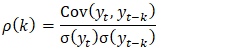(1)

Where represents the variance between the time series values at time t and time t-k and measures how much these values tend to vary together; is the standard deviation of the time series values at time t; and is the standard deviation of the time series values at time t-k. Similarly, the autocorrelation coefficient at lag k for a time series is given by equation (2).

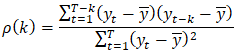(2)

Where is the mean of the time series; 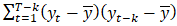computes the covariance between the time series values at time t and time t-k; and 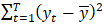computes the variance of the time series which measures the overall variability of the data. , represents the strength and direction of the linear relationship. If the autocorrelation is high (i.e. close to +1 or -1), it suggests a strong correlation between past and present values, demonstrating dependencies in the data. One of the fundamental features of a time series that can be identified through autocorrelation is stationarity.

3.1.2. Stationarity

A stationary time series is one whose statistical properties such as mean, variance and autocorrelation, do not change over time. Stationarity means that the time series does not have a trend or seasonality. The autocorrelation function (ACF) declines to near zero rapidly for a stationary time series whereas the ACF drops slowly for a non-stationary time series. There are two fundamental types of stationary time series. Strong stationary (i.e. strict stationary) and weak stationary. A time series is said to be strictly stationary if the joint distribution of is identical to that of 1. As a result, changing the origin time by lag k has no effect on the joint distribution. On the other hand, a time series is said to be weakly stationary provided: ; ;

Generally, data from real-life scenarios are mostly non-stationary. However, many time series models work under the assumption that the data is stationary. Consequently, the analysis of such model becomes more complicated when working with non-stationary data. One method to transform non-stationary data to stationary is by differencing. This method eliminates trends in the data. By using a difference operator, a non-stationary time series is transformed to a stationary time series. The difference of a time series is defined by equation (3).

(3)

Another way of stating the difference operator is by using a backshift operator (B) as defined in equation (4).

(4)

In equation (4) it is observed that the backshift operator (B) causes the data point it multiplies to be shifted backwards in time by 1 period.

Multiplication by higher powers of B correspondingly yields a backward shift by more than 1 period as given by equation (5).

(5)

Thus, multiplying by B to the kth power (i.e. lags k) has the effect of shifting a data point by k periods as given in equation (6).

(6)

The differencing operator can also be expressed in another form as given by equation (7).

(7)

Thus, the differenced series is obtained from the original series by multiplying by a factor of .

Now the second difference of is the first difference of and is given by equation (8).

(8)

In general, the kth difference of is obtained by multiplying by a factor of as given in equation (9).

(9)

A stationarity test needs to carried out in order to determine whether a time series has stable statistical properties over time. These tests are fundamental to modeling and forecasting time-series.

3.2. Statistical Tests

Statistical tests provide a quantitative approach to confirm or reject visual inspection findings. The Shapiro-Wilk test assesses whether a sample of data comes from a normally distributed population. Meanwhile the Augmented Dickey-Fuller and KPSS tests offer formal hypotheses for determining stationarity, helping us make objective decisions about appropriate modeling techniques.

3.2.1. Augmented Dickey-Fuller Test

The Augmented Dickey-Fuller (ADF) test is one of the methods to test whether the time series is stationary or not. The method is used to detect the unit roots in the time series data. A unit root refers to a stochastic trend in a time series, which shows an unpredictable systematic pattern. It is crucial to ensure that the variables are stationary since statistical inference assumes of constant means, variances and covariances. The ADF test has the following null and alternative hypotheses:

Null hypothesis (Ho): The time series is non-stationary,

Alternative hypothesis (Ha): The time series is stationary.

If the p-value is less than the chosen significance level then the null hypothesis is rejected and hence the time series is stationary. On the other hand, if the p-value is higher than the chosen significance level the null hypothesis is not rejected and hence the time series is non-stationary [36,37].

3.2.2. The Kwiatkowski-Phillips-Schmidt-Shin (KPSS) Test

The KPSS test is another method used to assess the stationarity of time series around a deterministic trend. The KPSS has the following null and alternative hypotheses:

Null hypothesis (Ho): The time series is trend stationary,

Alternative hypothesis (Ha): The time series is not trend-stationary.

If the p-value is higher than the chosen significance level the null hypothesis is not rejected and hence the time series is trend stationary. On the other hand, If the p-value is less than the chosen significance level then the null hypothesis is rejected and hence the time series is not trend-stationary. Thu, the time series is non-stationary which suggests that differencing is required [38].

3.2.3. Shapiro-Wilk Test for Normality

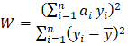
Generally, the assessment of the normality of a data set involves the use of a Q-Q plot, which gives a graphical visualisation of normality. If the data set scatter around the line of best fit inclined 45° with the horizontal-axis, the normality holds. However, a quantitative test is required to complement the visual inspection. The Shapiro-Wilk test is a hypothesis test that evaluates whether a data set is normally distributed. The Shapiro-Wilk test statistic (W) is defined by equation (10).

(10)

Where represents the number of observations; represents values of the ordered sample; and represents tabulated coefficients. The Shapiro-Wilk test has the following null and alternative hypotheses:

Null hypothesis (Ho): The sample belongs to a normal distribution,

Alternative hypothesis (Ha): The sample does not belong to a normal distribution.

For a 95% confidence interval, the Shapiro-Wilk test resulting in a p-value < 0.05, indicates that normality does not existence among residuals. On the other hand, a p-value > 0.05, indicates that the residuals are normally distributed [38].

3.3. Models for Stationary Time Series

3.3.1. White Noise Model

White noise model is the simplest time series model. Suppose is a white noise process, which is defined as a model whose random variable is independently and identically distributed. It is worth noting that for for , and for , for .

3.3.2. General linear model

For the general linear model each value of is a linear combination of both the current and preceding white noise processes and it is defined by equation (11).

(11)

Where represents the white noise process and denotes a series of constants such that

3.3.3. Autoregressive model

The autoregression processes are regressions on themselves. In an autoregressive model (AR(p) of order p, the model uses the p most recent values in the sequence to predict the next value. For example, an AR(1) model uses the two most recent values. An autoregressive model of order p at time t is defined by equation (12).

(12)

Where is a zero-mean white noise process with a standard deviation of .

3.3.4. Moving Average Model

A moving average model of order q (referred to as MA(q) uses past forecast errors in a regression-like model, rather than using past values of the forecast variable like an autoregressive model does. In a moving average model, each value of can be seen as a weighted moving average of the past few forecast errors. The model is defined by equation (13).

(13)

Where is a zero-mean white noise process with a standard deviation of are the moving average parameters, which results in different time series patterns when changed, and q is the order of the moving average [39].

3.3.5. Autoregressive Moving Average Model

Suppose the time series is an autoregressive moving average model of order p and q, denoted by ARMA (p, q) and defined by equation (14).

(14)

Where is a white noise process with a mean of zero and a standard deviation of . Notably, the ARMA process incorporates both AR and MA processes. It is interesting to note that if then equation (13) becomes an AR(p) process; however, if then equation (13) becomes an MA(q) model. In order to maintain a minimum order for p and q, AR(p) and MA(q) polynomials must have no common roots, where the AR(p) and MA(q) polynomials are defined by and , respectively.

3.3.6. Vector Autoregression Model

Vector autoregression (VAR) is used for multivariate time series (multiple related time series). Each variable in the system is modelled as a function of its own past values and the past values of all other variables in the system. The VAR model can be used to analyse relationships and predict future values across multiple related time series. A VAR model for a system of k variables and p lags, is represented by equation (15).

(15)

Where A k x 1 vector of endogenous variables at time t.

A k x k matrix of coefficients for each lag i.

A k x 1 vector of endogenous variables at lag t-i.

A k x 1 vector of error terms (white noise).

3.4. Hybrid VECM-ARIMA Model

Developing a hybrid VECM-ARIMA model involves a multi-step process that combines the techniques of vector error correction model (VECM) and autoregressive integrated moving average (ARIMA) models.

3.4.1. VECM Model

A VECM model is a specific type of Vector Autoregression (VAR) model, used when the time series are cointegrated. Cointegration implies that a linear combination of non-stationary time series gives a stationary time series. A VECM models the deviations from the long-run equilibrium, allowing for short-term adjustments to restore equilibrium. Thus, the VECM gives a combination of long-run equilibrium relationships and short-run dynamics. The general form of the VECM model is given by equation (16).

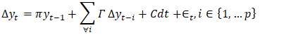(16)

Where Represents the first difference of the vector of variables at time t. This captures the short-run dynamics and could be the first difference of the dependent variable at time t.

The error correction term which represents the long-run equilibrium relationship between the variables. is a matrix that can be decomposed into where is the adjustment speed matrix and is the cointegrating vector, capturing the long-run relationships.

Represents the summation of lagged differences of the variables, capturing short-run dynamics and feedback effects.

Represents deterministic terms like constant or trend.

Represents the error term, assumed to be a vector of white noise with zero mean and constant covariance matrix.

The lag order of the model. This needs to be determined through model selection criteria like AIC, BIC etc. The sections 3.4.1.1, and 3.4.1.2 present essential steps in VECM modeling.

3.4.1.1. Data Pre-processing and Stationarity

Gather time series data for exogenous and endogenous variables and plot them to inspect for trends, seasonality, and outliers. Examine each time series for stationarity (constant mean and variance over time). Use techniques like ADF tests or visual inspection. Non-stationary series need to be differenced to achieve stationarity.

3.4.1.2. Cointegration Analysis

Fit a Vector Autoregression (VAR) model to the time series. Determine the optimal lag order for the VAR model using methods like the Akaike Information Criterion (AIC) or Bayesian Information Criterion (BIC) to minimize information criteria. Perform the Johansen cointegration test to determine if the variables have a long-run equilibrium relationship. This test will identify the number of cointegrating equations (relationships).

3.4.2. ARIMA model

The Autoregressive Integrated Moving Average (ARIMA) model integrates an AR and an MA model and thus combines differencing autoregression and moving average. ARIMA models are used to analyse and forecast individual time series data. They capture the autocorrelations within a single time series, meaning the dependence of a value on its past values. This model is denoted by ARIMA (p, d, q) where p is the order of the autoregressive (AR) component, representing the number of lagged terms used to predict the current value; d is the degree of differencing, indicating how many times the time series needs to be differenced to be stationary; and q is the order of the moving average (MA) component, representing the number of lagged forecast errors used to predict the current value. The general form of an ARIMA (p, d, q) model is given by equation (17).

(17)

Where The differenced time series at time t; The MA coefficients; The AR coefficients; and The white noise error term.

3.5. Model Evaluation Measurements

There are four different model evaluation measurements which are commonly used for evaluating and comparing different forecasting models.

3.5.1. Akaike Information Criterion

Akaike Information Criterion (AIC) is a single number score that can be used to determine measure of model fit, and thus which of multiple models is most likely to be the best model for a given data set. It estimates models relatively, meaning that AIC scores are only useful in comparison with other model AIC scores for the same data set. A lower AIC score indicates a better quality model (i.e. a better-fit model) [40]. The AIC is computed by equation (18).

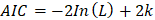(18)

Where is the Log-likelihood function of the model (i.e. A measure of how likely one is to see their observed data, given a model) and k is the number of parameters (number of exogenous variables) i.e. for ARMA (p, q) model. The Log-likelihood function is the logarithm of the Likelihood function.

Generally, the AIC works better for a large sample size as such it can potentially lead to a high degree of negative bias and overfitting when working with a small sample. To rectify this bias, a Corrected Akaike Information Criterion (AICc) is used. The AIC is a first-order estimate meanwhile AICc is the second-order AIC. The AICc is defined by an expression given by equation (19).

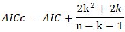(19)

Where n represents the sample size and k denotes the number of parameters.

3.5.2. Mean Absolute Error (MAE)

The Mean Absolute Error (MAE) refers to a measure of variability in the absolute values of distances between observations and their corresponding predicted values i.e. the average magnitude of the errors. The MAE is commonly used as a measure of prediction of errors and is therefore useful when evaluating forecasting models. The MAE is defined by equation (20).

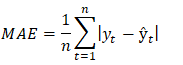(20)

Where n is the number of observations, is the actual observation and is the predicted value at time period t [35].

3.5.3. Mean Absolute Percentage Error (MAPE)

The Mean Absolute Percentage Error (MAPE) refers to a measure of variability in the absolute values of the ratio between the predicting errors and the observations. The MAPE is commonly used as a measure of prediction accuracy and is therefore useful when evaluating forecasting models. The MAPE is defined by an expression in equation (21).

(21)

Where n represents the number of observations, and represent the actual and the forecasted value at time period t respectively.

4. Application of Hybrid VECM-ARIMA Model for Evaluation and Forecasting of Carbon Emissions from Agrifood Waste Disposal systems in Tanzania

When applying the HVAM, the VECM captures the cointegration among multiple time series, and the ARIMA models capture the autocorrelations within each individual series. Specifically, the VECM model was applied in the analysis of the Tanzania’s agrifood supply chain to understand the short-run and long-run relationships between various variables influencing carbon emissions (kg tonnes) emanating from agrifood waste disposal systems. The exogenous variables that were analysed include agrifood processing activities, agrifood packaging activities, agrifood transportation, agrifood retailing activities, and agrifood household consumption whereas carbon emissions from agrifood waste disposal systems is an endogenous variable. On the other hand, ARIMA model was applied to forecast carbon emissions from the Tanzania’s agrifood waste disposal systems up to 2030 (i.e. In line with the United Nations SDGs). This allowed for identification of patterns and predicting future emission levels based on past trends. This study used secondary data retrieved from publicly accessible databases of Food and Agriculture Organization (FAO) and the Intergovernmental Panel on Climate Change (IPCC). The two sources offered historical datasets from 1990 to 2020.

4.1. Trends of Carbon Emissions and Statistical Tests of Variables in the Tanzania Agrifood Waste Disposal Systems

4.1.1. The Trend of Carbon Emissions from Agrifood Waste Disposal Systems over the Period 1990 - 2020

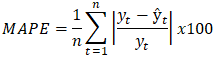
Figure 1 reveals an upward trend of emissions (kg tonnes of CO₂) from agrifood waste disposal systems over the period 1990-2020. The increase in emissions indicates a growing environmental degradation in agrifood waste disposal systems in Tanzania, most likely driven by the country’s population growth (i.e. from 26,206,012 in 1990 till 61,704,518 in 2020), expansion of agricultural production, and limited regulatory framework on green logistics and inadequacy of public awareness on environmental sustainability. Unless appropriate measures are taken by all parties in the green reverse logistics chain, the agrifood sector in Tanzania will continue to emit more GHGs which in turn raises global warming and climate change. Thus, reforms and optimisation measures are vital for facilitation of green economy which ultimately leads to the extenuation of climate change. Furthermore, understanding of emission trends, and the environmental impacts of agrifood waste disposal systems would disclose the opportunities and challenges to all stakeholders in the green reverse logistics chain of agrifood. In order to know whether stationarity exists, the time series data for agrifood waste disposal systems were subjected to ADF and Graphical test.

Figure 1. The trend of carbon emissions from Tanzania’s agrifood waste disposal systems over the period 1990 - 2020. (Source: Authors’ compilation from RStudio)

4.1.2. Stationarity Test

In order to know whether the time series data were stationary each variable was transformed in terms of the natural logarithm and apply the ADF test. The variables tested include Log(waste disposal), Log(food transport), Log(household consumption), Log(food retail), Log(food packaging), and Log(food processing). The results of the test before differencing the time series (I(0)) and after differencing the time series(I(1)) are shown in Table 1.

Table 1. ADF test at level l(0) and level l(1)

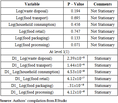
In Table 1, at level I(0) the for all variables, which implies that the time series is non-stationary since the null hypothesis (Ho) is not rejected. However, at level I(1) the 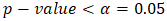for all variables, which implies that the time series is stationary since the null hypothesis (Ho) is rejected in favour of the alternative hypothesis (Ha).

4.1.3. Graphical Test of the Time Series Data

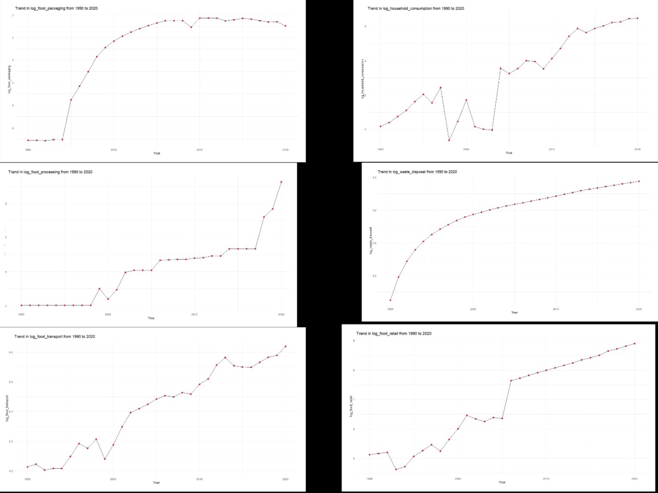
Visual inspection technique is crucial for assessing stationarity in time series data. It is a pictorial representation of the properties of the time series data. By plotting the time series and analyzing autocorrelation functions, it is possible to identify trends, seasonality, and changes in variance that indicate non-stationarity. Non-stationary series exhibit clear trends (upward or downward) or changing variance (increasing or decreasing spread) meanwhile stationary time series appears to have a constant mean (no clear trend) and variance (consistent spread) over time. Figures 2 and 3 depict the trend of all variables at level I(0) (i.e. before differencing the time series) and level I(1) (i.e. after differencing the time series) respectively.

From Figure 2 all of the variables show an upward trend. This means the mean and variance of each variable is changing over time hence the time series of each variable is not stationary at level l(0).

Figure 2. Trends of variables at level l(0) (Source: Authors’ compilation from Rstudio)

Figure 3 reveals that all variables have constant mean and variance over time, hence stationary at level l(1) i.e. after differencing the time series. Thus, the variation of each of these variables around its mean have a constant amplitude i.e. its short-term random time patterns always look the same in a statistical sense.

Figure 3. Trends of variables at level l(1) (Source: Authors’ compilation from RStudio)

4.1.4. Normality Test

The Shapiro-Wilk test was applied to test whether the residuals are normally distributed. All residuals for the six (6) variables were tested. These variables include Log(waste disposal), Log(food transport), Log(household consumption), Log(food retail), Log(food packaging), and Log(food processing). The values of W-statistic and p-values are indicated in Table 2.

Table 2. Results of Shapiro-Wilk test

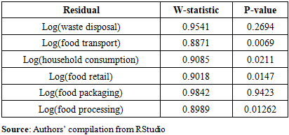
Since in Table 2 the for the two variables: Log(waste disposal) and Log(food packaging), the null hypothesis (Ho) is not rejected for these variables. This indicates that their residuals are normally distributed. In order to confirm the normality for the other variables, visual inspection of the residual plots is carried out.

4.1.5. Residual Plots

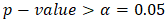
Figure 4 depicts the residual plots to visually test the normality for all variables.

Figure 4. Q-Q plots for normality test of variables (Source: Authors’ compilation from RStudio)

The residual plots in Figure 4, are aligned at 45° with the horizontal axis and the data points are scattered around the line of best fit, indicating that the normality holds for all variables. While the for the variables: Log(food transport), Log(household consumption), Log(food retail), and Log(food processing), suggesting statistically significant deviations from normality, their respective Q-Q plots display slight deviations from the line of best fit, which is not severe enough to invalidate the normality assumption.

4.1.6. Lag Order Selection

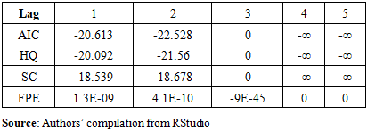
In order to determine the maximum lag for the model, the Akaike Information Criteria (AIC) was used considering its strengths over other criteria. It is worth noting that the chosen lag should be the one with the lowest AIC, as suggested by the RStudio program. The lag selection output and optimal value are shown in Table 3. From Table 3 it is clear that the optimal lag for the model is four.

Table 3. Lag selection output

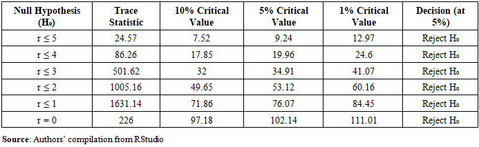
4.1.7. Cointegration Test

The Johansen test was applied to disclose the existence of long-run and short-run relationships between the endogenous variable (carbon emissions from agrifood waste disposal systems) and exogeneous variables (agrifood processing, agrifood packaging, agrifood transportation, agrifood retailing operations, and agrifood household consumption). The tested hypotheses were: Ho: There is no cointegration between variables, Ha: There is cointegration between variables. The tests results are presented in Table 4.

Table 4. Johansen test output

From Table 4, the trace statistic is greater than 5% critical value for all scenarios and thus the null hypothesis (Ho) is rejected for each case. The last rejection occurs at r ≤ 5 which implies that there are six (6) cointegrating relationships in the system. Consequently, there is long-run and short-run relationships between carbon emissions from agrifood waste disposal systems and agrifood processing, agrifood packaging, agrifood transportation, agrifood retailing, and agrifood household consumption.

4.2. Analysis of Carbon Emissions from Agrifood Waste Disposal Systems Based on VECM Model

Table 4 shows that all the variables: carbon emissions from agrifood waste disposal systems, agrifood processing, agrifood packaging, agrifood transportation, agrifood retailing operations, and agrifood household consumption are co-integrated. Thus, VECM model suits for this study.

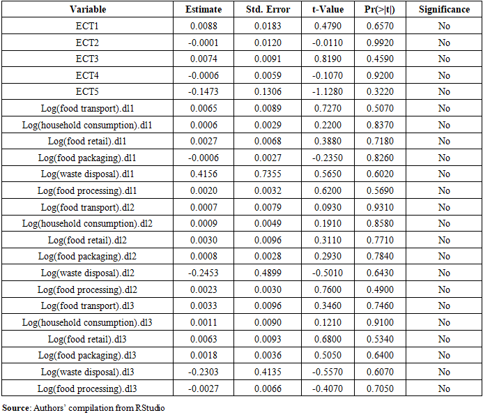
4.2.1. Short Run Dynamics

The short run dynamics are captured by the lagged differences of carbon emissions, which show how emissions in each sector respond to past changes in emissions from other sectors benefiting from agrifood. The results of the short-run dynamics are displayed in Table 5.

Table 5. Short run dynamics of lagged differences

From Table 5 it is revealed that no individual variable in the short-term has a statistically significant effect on carbon emissions from agrifood waste disposal systems. On the other hand, all ECTs are insignificant, suggesting slow or no adjustment towards long-run equilibrium in the short-run.

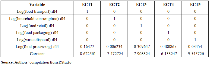
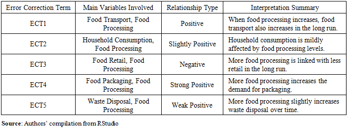
4.2.2. Long Run Effects

Table 6 reveals that all sectors except agrifood processing have a unit coefficient for their respective error correction terms (ECTs). In the long run, agrifood processing emerges the most influential sector on carbon emissions from agrifood waste disposal systems. To this end, deviations in carbon emissions from agrifood waste disposal systems are mostly corrected by changes in agrifood processing activities. These findings align with Smith et al. [6] who emphasise that agrifood processing activities are energy-intensive users. This is concomitant with the arguments of Love et al. [23] and Jehn et al. [12] that food processing significantly contributes to GHG emissions since is one of the most energy-intensive stages in the reverse logistics chain of agrifood. Thus, modernizing food processing plants with energy-efficient machinery and solar or hydroelectric power sources can significantly reduce carbon emissions. However, most SMEs in Tanzania’s agrofood industry lack capital and infrastructure to implement such changes [22]. Therefore, the government should play a key role by devising a variety of financing and fiscal schemes for SMEs.

Table 6. Long run effects

Similarly, from Table 6 it is worth noting that other exogenous variables including agrifood packaging activities, agrifood transportation, agrifood retailing operations, and agrifood household consumption exert insignificant long-run influence on carbon emissions from agrifood waste disposal systems, suggesting that they don’t serve as long-run anchors for stability of carbon emissions from agrifood waste disposal systems. However, these variables are still relevant for crafting sustainable policies. The model finds that different stages of Tanzania's agrofood supply chain are connected in the long run, especially through food processing as described in Table 7.

Table 7. Effect of ECT on variables’ relationship

Table 7 reveals that when agrifood processing increases, other variables like agrifood transport, agrifood packaging, and even carbon emissions from agrifood waste disposal systems are also affected, but at different rates. On the other hand, carbon emissions from agrifood waste disposal systems maintain a positive long-run relationship with food processing. Generally, more food processing leads to more waste, underlining the importance of integrating sustainable waste disposal systems into food manufacturer’s supply chains.

4.3. Forecasting of Carbon Emissions from Agrifood Waste Disposal Systems Using ARIMA Model

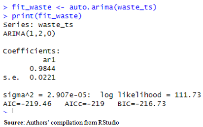
ARIMA model is a statistical analysis model that uses time-series data to either better understand the data set or to predict future trends through forecasting time series data [41]. More specifically, ARIMA models are the most general class of models for forecasting a time series which can be made to be stationary by differencing (if necessary), perhaps in conjunction with nonlinear transformations such as logging. This study applies ARIMA model to forecast carbon emissions from agrifood waste disposal systems up to 2030. It is worth noting that in order to achieve stationarity, the endogenous variable (i.e. carbon emissions from agrifood waste disposal systems) was transformed in terms of natural logarithm prior to model estimation and forecasting.

The Akaike Information Criteria (AIC) was used to choose the best ARIMA model for forecasting the endogenous variable. Table 8 reveals that ARIMA (1,2,0) was the most appropriate model for forecasting of carbon emissions from agrifood waste disposal systems.

Table 8. Auto selection ARIMA model

The ARIMA (1,2,0) provides a forecast of carbon emissions from agrifood waste disposal systems up to 2030 as depicted in Figure 5.

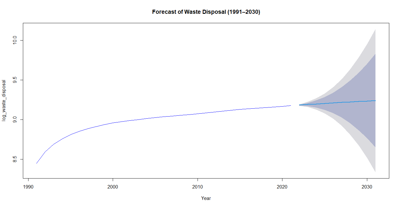Figure 5. ARIMA (1,2,0) forecast of emissions from agrifood waste disposal systems (Source: Authors’ compilation from RStudio)

Figure 5 shows that ARIMA forecast projects a slight increase in carbon emissions from 2020 to 2030. Albeit modest, the forecast indicates that if current environmental practices are improved, the trend of carbon emissions from agrifood waste disposal systems in Tanzania is talented. The findings are concomitant with the study by Sarfraz et al. [14] who predict the trend of CO₂ and CH₄ emissions from agricultural sector in China based on the historical data from 2000 to 2021 and demonstrate that the emissions will be constant in China for the next 10 years. This confirms the ongoing efforts to combat GHG emissions globally. Nevertheless, the stabilisation or slight increase in emissions is possible, provided green policies and regulations are formulated and adopted effectively, more energy efficient machineries and equipment are used in the agrifood supply chain, and stakeholder’s awareness continue to evolve. The control of carbon emissions from agrifood waste disposal systems are consistent with the attainment of most of the 17 United Nations Sustainable Development Goals (SDGs) including SDG 3 (Good health and well-being), SDG 7 (Affordable and clean energy), SDG 11 (Sustainable cities and communities), SDG 12 (Responsible consumption and production), SDG 13 (Climate action), and SDG 15 (Life on land). The findings are in line with the premise of an ongoing implementing measures to reduce agrifood waste emissions at all stages of the agrifood supply chain. Thus, deliberate efforts on emissions reduction are needed by all key stakeholders including farmers, food processors, transporters, distributors, retailers, consumers, government and environmentalists. Belamkar et al. [42] argue that any agrifood supply chain must optimise profit while minimizing CO₂ emissions. This argument is reinforced by Basri et al. [18] who point out the significant role of global food provision while shaping the quality of the environment to achieve carbon peak targets, carbon neutrality, and promote agricultural modernization. Yuniarti et al. [15] and Batool et al. [28] posit that integrating food production, distribution and waste recycling minimizes carbon emissions. Furthermore, reducing agrifood waste is therefore a crucial opportunity for sustainable innovation and climate action.

5. Conclusions

The objective of this study was to analyse and forecast carbon emissions emanating from the Tanzania’s agrifood waste disposal systems based on hybrid VECM-ARIMA model. The VECM model was applied to examine the short-run and long-run relationships between the study variables: agrifood processing activities, agrifood packaging activities, agrifood transportation, agrifood retailing activities, agrifood household consumption, and carbon emissions from agrifood waste disposal systems. The ARIMA model was applied to predict the Tanzania’s carbon emissions from agrifood waste disposal systems based on the data collected from FAO and IPCC over the time period from 1990 to 2020. The time series data were firstly subjected to the ADF test and found to be stationary after differencing. In addition, the stationarity of the time series for the exogenous and endogenous variables were confirmed by the visual inspection (i.e. graphical test).

The statistical tests were performed to examine the normality of data set and cointegration among variables. The Shapiro-Wilk test confirmed the normality for all variables. Meanwhile the Johansen test of cointegration revealed the existence of both long-run and short-run relationships between carbon emissions from agrifood waste disposal systems (i.e. endogenous variable) and agrifood processing activities, agrifood packaging activities, agrifood transportation, agrifood retailing operations, and agrifood household consumption (i.e. exogeneous variables). More specifically, the short-run dynamics revealed that no variable posed a statistically significant influence on carbon emissions from agrifood waste disposal systems. In the long-run, only agrifood processing activities exerted a statistically significant influence on carbon emissions from agrifood waste disposal systems since its Error Correction Term (ECT) is non-zero. On the other hand, the Criteria Akaike Information Criteria (AIC) was used to choose ARIMA (1,2,0) which provided a forecast of carbon emissions from agrifood waste disposal systems over the period 2020-2030. The ARIMA forecasting model revealed a slightly decline of the growth rate of carbon emissions from agrifood waste disposal systems up to the year 2030. This suggests that emission mitigation measures in the agrifood supply chain are being implemented. Furthermore, understanding the intricate connection between sub-systems of the agrifood supply chain and agrifood waste disposal systems is crucial for informing all stakeholders about the opportunities and challenges associated with the mitigation of GHG emissions in the food sector. Specifically, the minimization of the impact of carbon emissions from agrifood waste disposal systems is guaranteed provided green policies and regulations, green technology and stakeholders’ awareness towards sustainable supply chains continue to evolve. Furthermore, this study can serve as guidance for other countries where carbon emissions from agrifood waste disposal systems are still escalating.

5.1. Implications for Research

The findings of the study have theoretical, practical, and social implications. Theoretically, this study appears to be the first to provide a comprehensive VECM-ARIMA model that analyses concurrently carbon emissions from agrifood waste disposal systems attributed by agrifood supply chain components including agrifood processing activities, agrifood packaging activities, agrifood transportation, agrifood retailing activities, and agrifood household consumption. The tendency has been to model one or few of these agrifood supply chain components and thus provided limited understanding on carbon emissions from agrifood waste disposal systems. The actors in the agrifood reverse logistics chain have typically focussed on economic sustainability (i.e. cost reduction) while environmental sustainability has received less attention. In addition, the study adds theoretical knowledge with regard to agrifood supply chain emissions. Practically, results shed light on what all parties to the agrifood reverse logistics chain are supposed to take in order to curb carbon emissions and support the UN sustainable development goals while considering the escalating society’s demands on green supply chain. Specifically, this study makes all parties aware of their contribution to carbon emissions from agrifood waste disposal systems (i.e. farmers, food processors, transporters, distributors, retailers, consumers and the government) which in turn enables them to formulate strategies which would minimize the pollution of carbon emissions. This work helps the policy makers in developing effective policies regarding the management of agrifood waste in a sustainable manner. Socially, this study is resourceful for people, society and underprivileged. The savings resulting from emissions reduction will accrue to the society in various forms including increase in budget for food security and social affairs.

5.2. Limitations and Directions for Future Research

While this study discloses valuable insights into the analysis and prediction of carbon emissions associated with the Tanzania’s agrifood waste disposal systems, it still suffers from several limitations. Firstly, agrifood supply chain originates from crop cultivation (in fact land preparation) till the point when agrifood waste is disposed. It is evident that this study excluded some of sub-systems (i.e. crop cultivation, pesticides manufacturing, fertilizers manufacturing, manure management) in order to simplify the model. Secondly, VECM-ARIMA model while powerful for time series analysis, each have limitations. VECM model struggles with high dimensionality and requires large datasets for accurate estimation. ARIMA models on the other hand, are limited to linear relationships, struggle with non-stationary data requiring manual transformations, and may not be suitable for long-term forecasting. Nevertheless, the study provides in-depth and significant insights to the farmers, agrifood equipment suppliers, agrifood processors, agrifood transporters, agrifood distributors, agrifood retailers, agrifood consumers, and other stakeholders interested in deeper understanding of green supply chains. Future studies should incorporate more parameters including modeling the interaction of upstream activities (e.g. crop cultivation, on-farm energy use, pesticides manufacturing) and carbon emissions from agrifood waste disposal systems to give more reliable results and generalizability.

Declarations

All authors declare that they have no conflicts of interest.