B. Vara Prasad Rao1, K. Gangadhara Rao2
1Department of Computer Science & Engineering, R.V.R & J.C College of Engineering, Chowdavaram, Guntur, Andhra Pradesh, India
2Department of Computer Science & Engineering, Acharya Nagarjuna University, Guntur, Andhra Pradesh, India
Correspondence to: B. Vara Prasad Rao, Department of Computer Science & Engineering, R.V.R & J.C College of Engineering, Chowdavaram, Guntur, Andhra Pradesh, India.
| Email: |  |
Copyright © 2017 Scientific & Academic Publishing. All Rights Reserved.
This work is licensed under the Creative Commons Attribution International License (CC BY).
http://creativecommons.org/licenses/by/4.0/

Abstract
A Non Homogenous Poisson Process (NHPP) with its mean value function generated by the cumulative distribution function of linear failure rate distribution is considered. We consider some truncated time values and use them in the mean value function of NHPP. The variation of the original mean value function and the mean value function at the truncated time is considered. A decision is taken to stop testing the software based on the difference between the mean value function and the mean value function at the truncated time. Truncated reliability aspects are discussed using four data sets.
Keywords:
SRGM, RELEASE TIME
Cite this paper: B. Vara Prasad Rao, K. Gangadhara Rao, Truncated Software Reliability Growth Model Based on Linear Failure Rate Model - Release Time Policy, Journal of Safety Engineering, Vol. 6 No. 1, 2017, pp. 1-7. doi: 10.5923/j.safety.20170601.01.
1. Introduction
In the theory of probability, F(t) is called the cumulative distribution function (CDF) of a continuous non-negative valued random variable. Thus an NHPP designed to study the failure process of a software can be constructed as a Poisson process with mean value function based on the cumulative distribution function of a continuous positive valued random variable. If a software system when put to use fails with probability F(t) before time t, if 'a' stands for the unknown eventual number of failures that it is likely to experience, then the average number of failures expected to be experienced before time t is a.F(t). Hence a.F(t) can be taken as the mean value function of an NHPP. We know that the cumulative distribution function (cdf) of the linear failure rate distribution is given by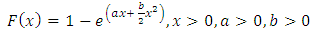 | (1.1) |
The NHPP with F(θ,x) as the mean value function is prepared by us as the SRGM for our present study.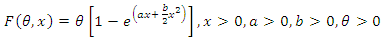 | (1.2) |
Cumulative distribution functions of positive valued random variables play an important role in the development of software reliability growth models through non-homogenous Poisson process (NHPP) in Pham (2000) [2]. The notion of NHPP with cumulative distribution function of LFRD along with the concept of truncation is used in this work in an admissible way to decide the point of truncation on one hand and the optimal release time of the software product in a di erent sense. The suggested procedure is illustrated for four different data sets also. The rest of the paper is organized as follows. Evaluation of the mean value function by moment type method of estimation of statistical science given by Kantam et al. (2014) [1] is briefly presented in section 2. Our suggested procedure for the estimated mean value function to a hypothetical data set is described by section 3. The illustration of the results of our procedure for live data sets is presented in section 4. Summary and conclusions are given in section 5.
2. Moment Type Method of Estimation
The parameters of the mean value function generated by NHPP using LFRD model requires estimation because they are generally unknown. The most frequently used classical method of estimation is the well known Maximum likelihood method. However for LFRD model this method does not yield analytical solutions. As an alternative Kantam et al. (2014) [1] suggested a simpler, efficient ready to use method called moment type method of estimation and provided auxiliary tables for immediate use overcoming numerical iterative procedures. For the sake of theoretical justication the moment type method of estimation is briefly in this section. This method applied to any data gives the estimation of parameters the mean value function which is essential for a suggested procedure described in section 3.In the present paper we consider the CDF of LFRD as the genesis of mean value function of our SRGM. All these models are either constant failure rate (CFR) or of absolutely instantatenous failure rate (IFR). In the theory of distributions a com-bination of exponential distribution which is CFR model and Rayleigh which is IFR model is used through hazard function to get a model called LFRD whose hazard function is a perfectly increasing straight line of the form y=a+bx. Such a distribution is proved to be having a number of important applications in survival analysis, a proxy concept to reliability theory with a view to model software failure data with LFRD. We consider the pdf.The probability density function (pdf) of Linear Failure Rate Distribution is given by | (2.1) |
Its cumulative distribution function (cdf) is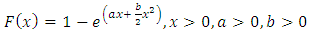 | (2.2) |
The NHPP with F(θ,x) as the mean value function is prepared by us as the SRGM for our present study.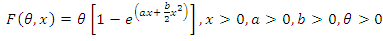 | (2.3) |
Thus our proposed SRGM contains 3 parameters namely θ, a, b where θ stands for the unknown number of faults latent in the software. It is also the limiting value of the mean value function as tà∞. For any general NHPP representing as SRGM the software reliability is given by | (2.4) |
which is the probability of zero failures between the time t to t+x where t is the execution time of the software during which testing was done and x is additional time period upto which the user wants the software to function failure free. The quality of the software is based on the magnitude of the software reliability. We can know it only if the parameters of SRGM are known and t,x are specified. But generally, the parameters remain unknown and need to be estimated with the help of software failure data. Usually, the parameters will be estimated using the classical M.L. method. The loglikelihood equations to get the MLEs of the parameter after simplification for LFRD generated SRGM are: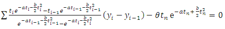 | (2.5) |
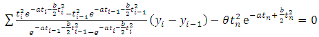 | (2.6) |
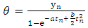 | (2.7) |
In view of the complicated nature to get the solutions of loglikelihood equations, we resort to moment type of estimation of the parameters as provided in kantam et al (2014) [1]. For a ready reference this method is presented below briefly:The Mean, Variance and coefficient of variation (CV) of a reparameterised LFRD are respectively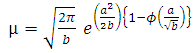 | (2.8) |
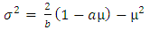 | (2.9) |
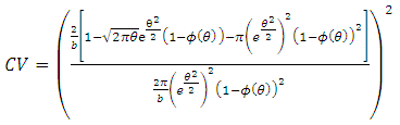 | (2.10) |
where ϕ(θ) is cumulative distribution function of standard normal distribution. It can be seen that from equation (2.10) that there is a one-one correspondence between the population CV and θ of reparameterised LFRD. This motivates us to develop an auxiliary table between various hypothetical values of and CV expressed by equation (2.10). In fact the RHS of equation (2.10) is evaluated for various values of =0(0.001)0.5, so that for any live value of coefficient of variation (CV) one can get back the corresponding θ, with interpolation if necessary. A part of the values corresponding to =0(0.001)0.5 is listed in the table 1. The remaining values are available with the authors.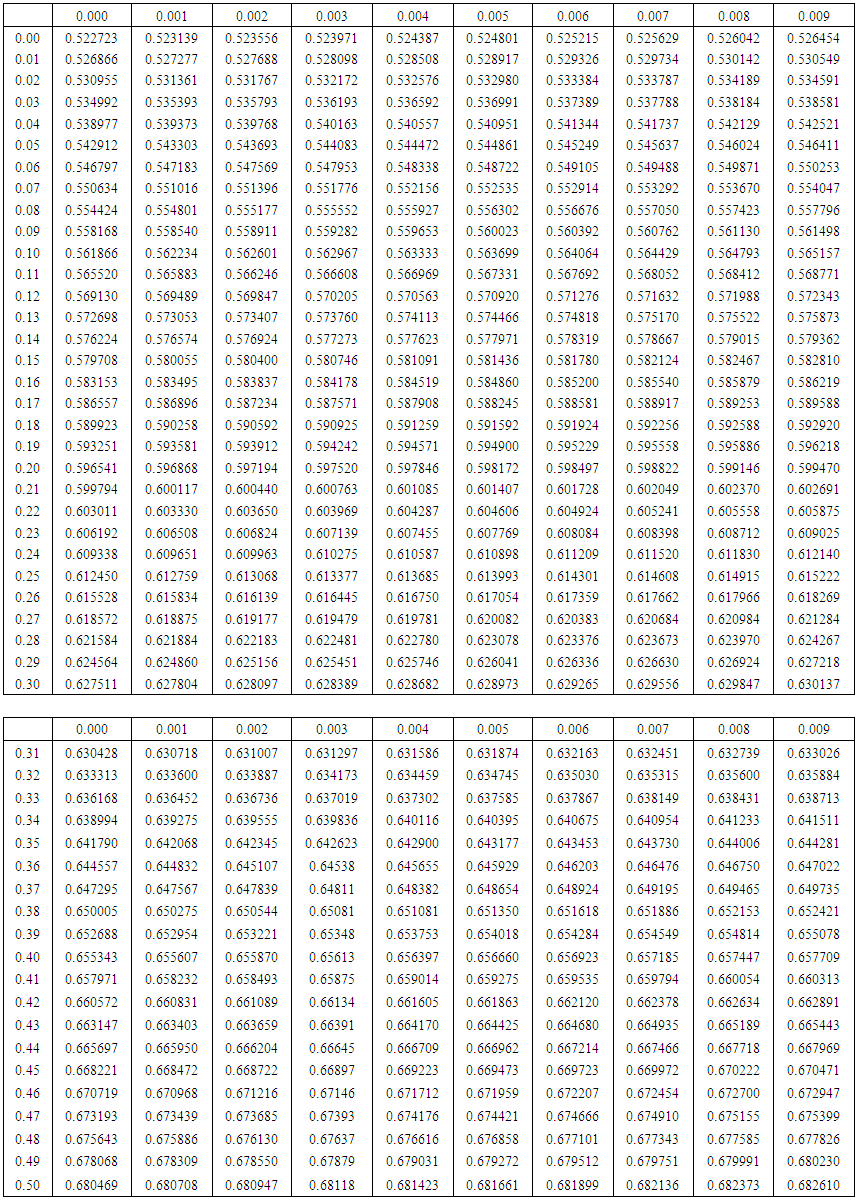 | Table 1. Auxiliary Table of CV for a given θ |
3. Procedure to Determine Truncated Point
It is well known that a typical software failure data set shall be of the form (ti,yi), i=1,2,..,k. where ti is the time and yi is the number of failures experienced by a software up to time ti, also t1 < t2 < ::: < tk. In our procedure we take the first two time incidents initially say (t1,t2) and define a hypothetical truncated time for this subset as something more than t2 say T1. Using the time point (t1,t2) the parameters of the mean value function are estimated by the method described in section 2. These estimates would give the estimated values of the mean value function at (t1; t2; T1).The absolute difference of |m(t2) - m(T1)| is noted down say A1.The data is now supplemented by the next two time points namely (t3; t4) thus having a data set of four time points t1 < t2 < t3 < t4 in a moving manner. For this supplemented data set another hypothetical truncation time say T2 typically more than t4 is taken. As described above the parameters are estimated using t1 to t4 and the absolute difference between |m(t4) - m(T2)| say A2 is noted down.This procedure is repeated each time supplementing the data by the successive pairs of time incidents ti, ti+1 and estimating the corresponding absolute difference Al at the ith time till all the time points up to tk are exhausted. For a given data set the graph of Al against l (l=1,2,...) shows a trend of falling down and raising at a particular l where the direction is changed is identi ed and the maximum ti of the time points used at that stage is recommended as the suitable point of truncation. That point may be taken as the optimum release time of the software product and also the termination time at the software testing. This procedure is applied to four data sets as illustration and is given in section 4.
4. Illustration
Four different data sets published in Wood (1996) [3] and Pham (2005) [4] are considered for illustration of the above procedure to determine the truncation point. The last row presented in the table of each data set indicates Al values. The place at l where the trend of Al changes its direction is shown in bold type. At that place in the column of tis the largest ti is recommended as truncation time also marked in bold type which in our proposal as the optimal release time / stoppage rule of the software testing.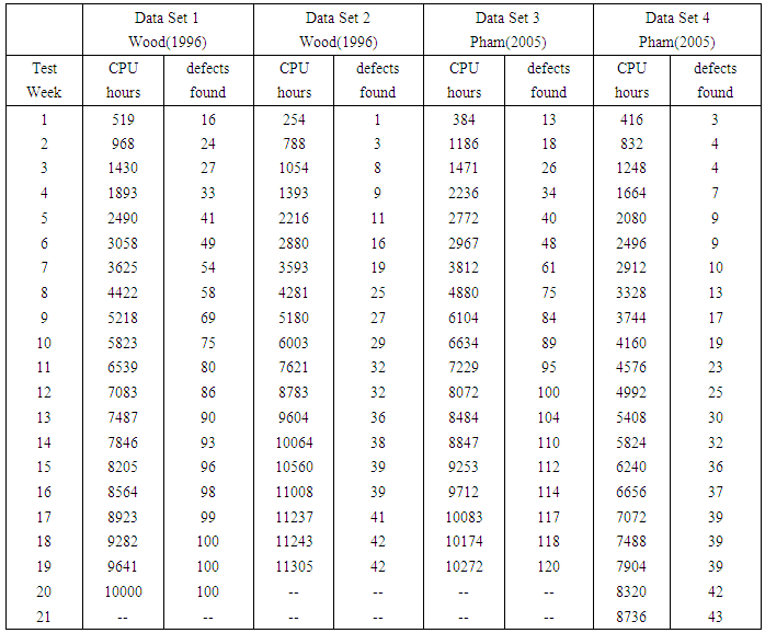 | Table 2. Data Sets |
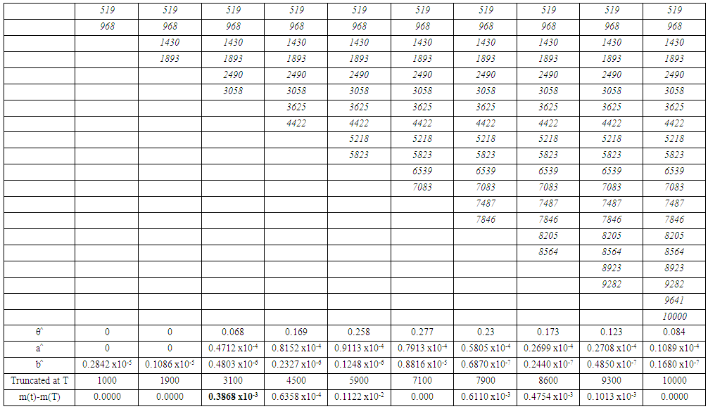 | Table 3. Difference table of m(t)-m(T) for Data Set 1 |
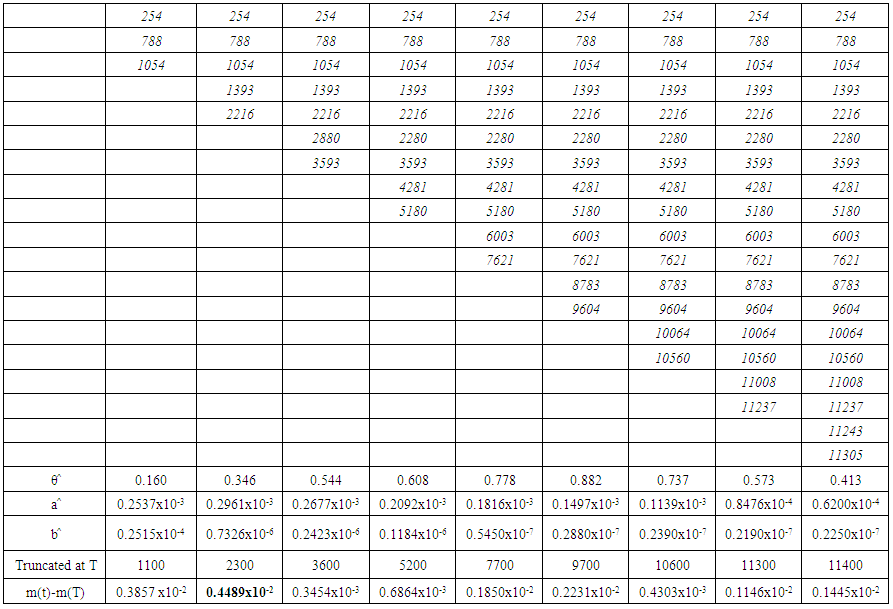 | Table 4. Difference table of m(t)-m(T) for Data Set 2 |
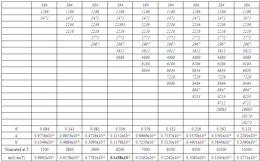 | Table 5. Difference table of m(t)-m(T) for Data Set 3 |
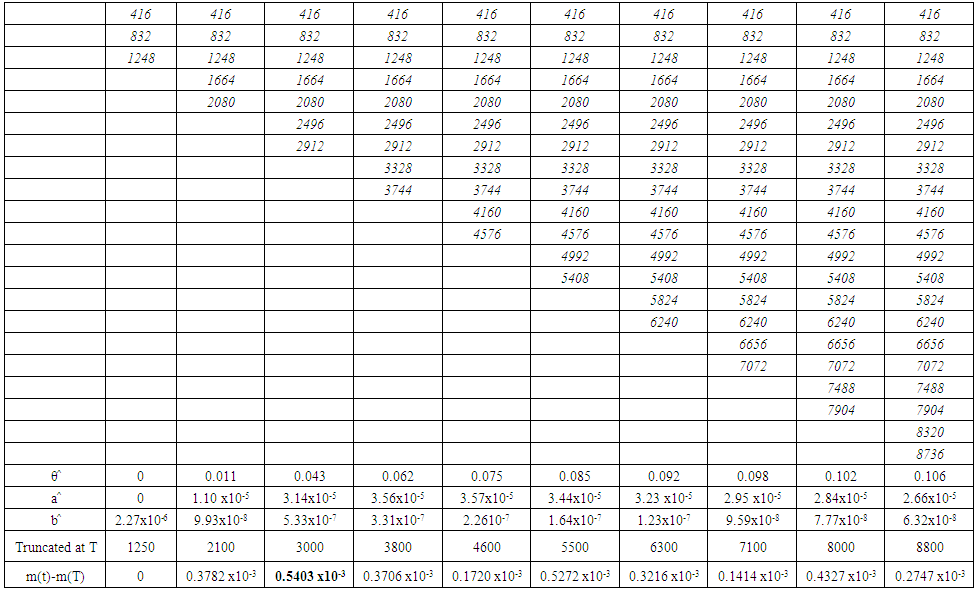 | Table 6. Difference table of m(t)-m(T) for Data Set 4 |
Graphs indicating release time based on the mean value function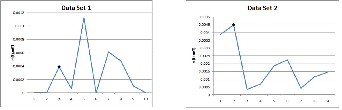 | Figure 1 & Figure 2 |
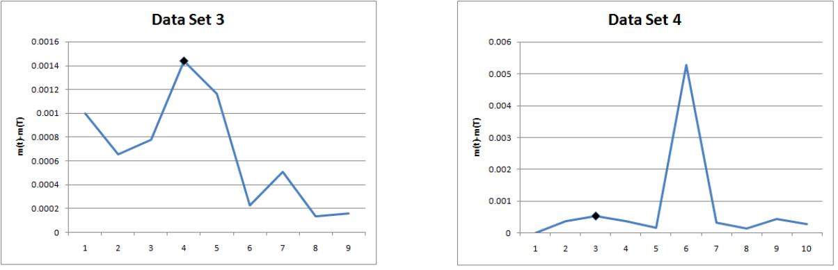 | Figure 3 & Figure 4 |
5. Summary & Conclusions
In software testing processes testing time is a key aspect. It is desirable to suggest a time point where testing is to be terminated and the product is to be released. In such situations a admissible stoppage rule is necessary to save the time aspect. The notion of truncation is used in this work to suggest optimal stoppage rule for a software product assuming that the failure phenomenon of the product is described by our NHPP with LFRD cdf as its mean value function. The method we suggested is simpler in mathematics without sacri cing its precision and can be readily used by practitioners to arrive at the stopping rule of the experiment.
References
| [1] | Kantam. R. R. L., Priya. M. Ch., and Ravikumar. M. S Moment type estimation in linear failure rate distribution. IAPQR Transactions, 39(1):87-97, 2014. |
| [2] | Pham. H. Software Reliability. Springer-Verlag, 2000. |
| [3] | Wood. A. P. Predicting software reliability. IEEE Computer, 11:69-77, 1996. |
| [4] | Hoang Pham. A generalized logistic software reliability growth model. Operational Research Society of India (OPSEARCH), 42(4): 322-331, Dec 2005. |

 Abstract
 Reference
 Full-Text PDF
 Full-text HTML