1. Introduction

Reliability is the probability that a system/component works properly during specific times under specific environment conditions. Two general approaches can be followed to increase the system reliability through increasing the component reliability or by adding redundant components. Adding redundant components is variously called redundancy optimization, redundancy allocation or reliability redundancy allocation problem (RRAP). RRAP is an optimization problem that is comprised of either reliability or cost, or both of them, as objective functions. Some common constraints such as cost, volume and weight of components and system are investigated in this approach.

In previous researches, meta-heuristic methods have been widely applied to solve redundancy optimization models. Reference[1] stated that the behaviour of components is not always specific and is variable over time. As a result, they used interval values for presenting component reliability, and applied GA for solving the developed model on series systems. Reference[2] developed a mathematical model that its objective function was to maximize reliability of the system. The constraints were upper limits of the cost, volume and weight of the system. They investigated two cases called as complex (bridge) system and over speed protection system for a gas turbine. In the research, a hybrid approach including PSO, Gaussian probability distribution and chaotic sequence is applied to solve the proposed model. Reference[3] considered three redundancy optimization models in series condition. The first model tried to minimize cost by regarding lower limit of the system reliability as a constraint. The second model maximized system reliability when cost of the system does not exceed an upper bound. The third model maximized system reliability when cost and weight of the system do not exceed their upper bounds. They applied a hybrid algorithm by using genetic algorithm and simulated annealing to solve examples of the three proposed models.

Reference[4] proposed a multi-objective model including redundancy, reliability and life cycle cost simultaneously as objective functions. NSGA2 is applied to solve some application examples of the model to specify optimum maintenance program. Reference[5] examined some examples of redundancy allocation problem with linear and nonlinear constraints. They applied a penalty function approach to search in both feasible and infeasible spaces to reach a near optimal solution. At the end, they showed the superiority of the proposed procedure by comparing the results they reached with those of previous researches. Reference[6] focused on solving redundancy optimization by a proposed branch and bound (BB) method. The proposed method was adaptable to either of linear or nonlinear, single or multi constraints, and convex or concave problems. At the end, the comparisons showed the better performance of the developed approach relative to the previous exact methods. Reference[7] applied simulated annealing (SA) method to assign redundancy and reliability levels to the subsystems in series, series-parallel and bridge systems. Reference[8] examined multi-objective redundancy allocation problem in series-parallel systems. The developed model had system reliability and designing cost as objective functions and weight of the system as a constraint. They applied MOEA and NSGA-2 approaches to solve the developed model. Reference[9] studied a model that included maximizing system reliability, and minimizing cost and weight as objective functions. They used Tabu Search (TS) method to find Pareto set of efficient solutions of multi-objective redundancy allocation problem. After that Pareto front pruning Monte-Carlo simulation were used to prioritize Pareto front solutions and specify promising solutions.

Reference[10] investigated three multi-objective models including reliability, cost and weight as objective functions. Variable neighborhood search (VNS) algorithm was applied to solve the developed models. Reference[11] regarded availability maximization and cost minimization as two objective functions of a model. Also, they considered that the cost of each component depended upon the failure rate and repair rate. For solving the developed model, two objective functions were transformed to a single objective function and then genetic algorithm was used to solve the single objective problem. Reference[12] investigated system reliability, cost, volume and weight as fuzzy goals. Several numerical examples of the developed models were solved by having various kinds of aggregators and using threshold accepting algorithm. Reference[13] studied three types of multi-objective optimization problems including cost, reliability and weight factors. They applied simulated annealing method to solve the problems. Reference[14] studied multi-objective problems by taking into account maximizing system reliability estimation and minimizing the variance of system reliability estimation. Efficient solutions were found by solving a series of multi-objective problems. Reference[15] applied dynamic programming and Hooke–Jeeves pattern search to present a combined model for redundancy allocation problem that minimized cost as an objective function. Reference[16] added a new decision variable to redundancy allocation problem that specified type of redundancy (active or cold). Afterwards, genetic algorithm was applied for solving the developed model.

Most of the previous researches have focused on different methods to solve redundancy optimization problem. In this article, however, an approach is developed by using some aspects that have not been viewed in other researches. The first aspect considers reliability level of each component as a fuzzy triangular number. The second aspect concerns the cost discount rate of the components. Discount rate is the one that is provided by suppliers in cases of buying products in high volumes.

The mathematical model that includes the specified features is developed in section 2 below. The single and multi-objective particle swarm optimization method is explained in Section 3. Constraint handling strategy for solving the proposed model is stated in section 4. The computational results are given in section 4 and include two examples and their results. Finally, the last section is devoted to the conclusions and suggestions for future researches.

2. Problem Definition

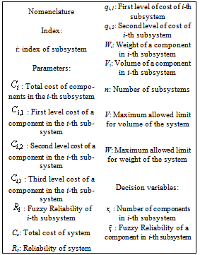
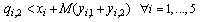
In this section the mathematical model of a reliability redundancy allocation problem is stated. Often, reliability of a component is not specific. There are many reasons for this issue that are: (a) Reliability depends on operational conditions and environment. Therefore, it is not possible to determine a fixed number that shows reliability of a component in all conditions; (b) reliability may be taken into account in design phase. In this phase, it is difficult to determine reliability specifically; (c) It is probable that the component is relatively new and there would be no data about component failures and time to failures. Consequently, there is no certain parameter for reliability, allowing it to be regarded as an inaccurate parameter. Fuzzy theory can help to effectively handle these parameters. In this research, reliability of a component is regarded as a triangular fuzzy number. Indices, parameters and decision variables are stated as follows.

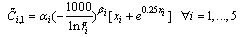
Discount rate is the second differentiation in this research. In the previous researches, cost of components was not related to the number of components. But, in real world, by increasing the number of components their cost is usually decreased through applying different conditions for discount rate. In this research, overall discount is applied and defined in three levels as follows.

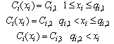Where

Objective functions

(1)

(2)

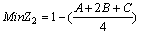
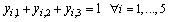
Two objective functions indicate minimizing overall cost and maximizing overall reliability of the system respectively. For consistency between objectives, is taken as second objective function. It results in that both of the objective functions are about minimizing.

Constraints

(3)

(4)

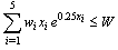
(5)

(6)

(7)

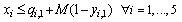
(8)

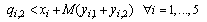
(9)

(10)

(11)

(12)

(13)

(14)

(15)

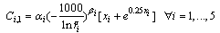
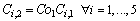
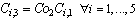
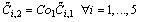
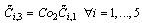
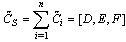
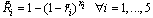
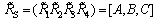
Constraints (3) and (4) concern that volume and weight of the system are not greater than specific limits. Constraints (5) to (8) specify that the number of components in each subsystem is placed in intervals in order to compute cost and discount of the components. In this article, and are equal to 2 and 4, respectively, to show the three levels of discounting. Constraint (9) computes the cost of components in each subsystem on the bases of the number and reliability of components. Constraints (10) and (11) compute the cost discount of components. 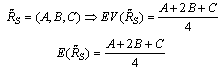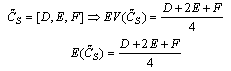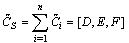In this article, and are supposed to be 0.9 and 0.8 respectively. Constraints (12) and (13) calculate the cost of each subsystem and the cost of the system respectively, giving as well the cost of the system as a triangular fuzzy number. Constraint (14) computes reliability of each subsystem on the bases of the number and reliability of components. Constraint (15) computes reliability of the system. Function f is structure function of the system that measures the reliability of the whole system using reliability of subsystems.

For solving the developed fuzzy model, it is necessary to convert it to a crisp model. Since the reliability of each component is considered as a triangular fuzzy number, reliability of subsystems and reliability of system is a triangular fuzzy number too.

Reliability of a component is supposed as a triangular fuzzy number like[a, b, c]. a and c are specified by difference of them with b. For i-th component, a, b, c are shown by (r_i-I), (r_i) and (r_i+I) and reliability of that component is a triangular fuzzy number like[r_i-I, r_i, r_i+I]. Therefore, reliability of each subsystem is obtained as below.

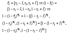(16)

The concept of expected value[17] is used to convert this triangular fuzzy number to a crisp number. The expected value is shown by EV.

(17)

Since the cost of each component is related to the reliability, cost of each component, subsystem and system is a triangular fuzzy number.

(18)

Figure 1 Depicts the flowchart of the proposed approach for solving RRAP in this research.

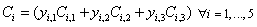
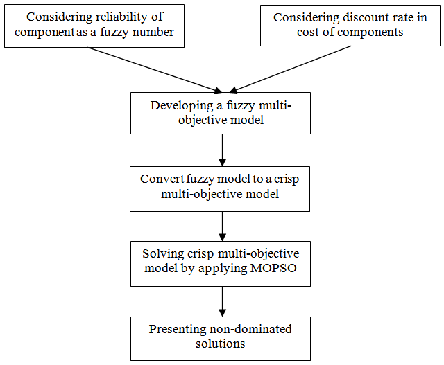Figure 1. Flowchart of the proposed approach for solving RRAP

3. Multi-Objectives Particle Swarm Optimization

3.1. General

Particle swarm optimization (PSO) is a meta-heuristic method that is used to solve optimization problems efficiently. In this method, first, an initial swarm that includes a number of particles is created. Each particle shows one solution of the problem and has a position and a velocity that are changed in each iteration to obtain better solutions. During iterations, the best position of each particle (that maximizes or minimizes objective function) is saved in a variable such as pbest. The best position of all of particles is saved in a variable that is called gbest. The parameters and variable in PSO are shown below.

x_i,1, x_i,2, …, x_i,n: n continuous decision variables

x_i=[x_i,1, x_i,2, …, x_i,n]: Position vector in the i-th iteration.

v_i=[v_i,1, v_i,2, …, v_i,n]: Velocity vector in the i-th iteration.

pbest_i: Vector that stores the best position of the particles during iterations

gbest_i: Best positions of all particles during iterations

c₁, c₂ : Predefined coefficients

r₁ and r₂: Random numbers between zero and one.

w: Inertia factor that is equal to 0.4

In this article, each solution has two parts. The first part includes number of components in subsystems. The second part includes reliability of component. For example, a typical solution for a system with four subsystems appears as shown below.

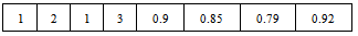The above solution explains a system with four subsystems that include 1, 2, 1 and 3 components. Reliabilities of components are 0.9, 0.85, 0.79 and 0.92 respectively. The above solution includes discrete and continuous numbers. Since PSO handles continuous numbers easily, it is necessary to modify solution in order to be consistent with PSO approach. Therefore, if the number of components is a continuous value, it is rounded to an integer number. For example, 2.4 and 3.7 are converted to 2 and 4 respectively. If the number of components in a subsystem is smaller than one, it is rounded to one.

In this approach, multi-objective PSO (MOPSO) is used to solve reliability redundancy allocation problem[18]. In MOPSO a crowding distance (CD) factor is defined[15] to show how much a non-dominated solution is crowded with other solutions. Consider a set of solutions including k non-dominated ones. It is possible to calculate CD factor for each solution as follows. (a) First, it is necessary to sort solutions in an ascending order for each objective function; (b) CD factor of the first and last solution is equal to a big number like M; (c) For the other solutions, CD factor is calculated by following relation.

(19)

(d) The overall CD factor for each solution is equal to sum of CD factors of all objective functions of that solution.

3.2. MOPSO Algorithm

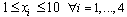
MOPSO algorithm is defined through the following steps for the RRAP:

Step 1: first, initial swarm of particles is generated. It is usually done randomly. For reliability of a component, a random number between 0 and 1 is generated; likewise, a random number between 1 and 10 is generated for number of components in a subsystem. The initial velocities of particles are set to zero as well.

Step 2: all particles are examined, and non-dominated solutions from swarm are selected and stored in a collection that is named repository. In each iteration, repository is updated and new non-dominated solutions are added to. Then, current solutions of repository are examined and if any of them is dominated by new solutions, it will be deleted from repository. Note that the capacity of repository is limited and is specified by a predefined parameter. If the number of non-dominated solutions is more than the capacity of repository, number of solutions is reduced as a result by using crowding distance (CD) factor that is defined previously. Based on this approach, solutions with smaller CD factors are deleted. Consequently, solutions in less crowded spaces remain in repository.

Step 3: pbest of each particle is equal to its initial position in the first iteration. In the next iterations, pbest for each particle is computed based on the following rules:

1) If the current solution is dominated by the pbest solution, then pbest solution remains unchanged.

2) If the pbest solution is dominated by the current solution, then the current solution is stored as pbest.

3) Otherwise, one solution is selected as pbest at random.

Step 4: In each iteration, the velocity of each particle is computed by this equation:

(20)

Note that gbest in velocity equation of single objective problem is replaced by rep_H in velocity equation of multi-objective problems. rep_H indicates one of the solutions that is selected from repository. In this it is selected here randomly from less 10% crowded solutions.

Step 5: The new position of each particle is attained by using this equation:

(21)

Step 6: steps (1) to (5) are repeated until the number of iterations reaches to the number that is specified before.

It is necessary to mention here that in this article each swarm includes 20 particles, MOPSO approach is repeated 50 times and capacity of repository is equal to 50. The constant coefficients in velocity equation (c₁ and c₂) are set to 2.

4. Constraint Handling Strategy

Constraint handling is an important issue in meta-heuristic methods that includes four different strategies. The strategies are: (a) Reject: this strategy rejects every infeasible solution; (b) Modify: in this case the structure of solution is designed as always feasible solutions are generated. (c) Repair: in this strategy each infeasible solution is changed to reach to a feasible solution. (d) Penalty function: this approach accepts infeasible solutions by assigning them a penalty function.

In this article repair strategy is used by applying different approaches on different conditions as stated below:

A) If volume and weight constraints are violated, then one of the subsystems is selected at random. If the number of components in the subsystem is greater than one, then it is reduced by one.

B) If constraint about number of components is violated, then a simple approach is used. If number of components is smaller than their lower specified limit, then the number of components is set to the lower limit of the components. Similarly, if the number of components is greater than their upper specified limit, then the number of components is set to the upper limit.

C) Suppose that there are violated constraints about reliability of components. If reliability of a component is less than lower specified limit, it is set to the lower limit. Also, if reliability of a component is greater than upper specified limit, a new random number is generated and is assigned to the reliability of the component.

The above-mentioned three rules are applied until a feasible solution is attained. Then, infeasible solution is replaced by the attained feasible solution.

5. Computational Results

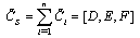
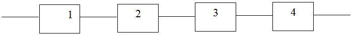
To show the efficiency and applicability of the proposed approach, two examples from Coelho[2] are selected and solved. These examples include reliability as objective function and cost, volume and weight of the system as constraints. Since the developed approach in this research concerns multi-objective function, it is necessary to modify the examples to be consistent with the proposed framework in the present article. To this end, cost and reliability of system are regarded as objective functions. Also, reliability of the components is taken as a triangular fuzzy number, and cost of the components is stated in three levels by taking account discount rates. By this approach, the modified examples are stated and solved as shown below.

Example 1 (A bridge system)

The first example is about a bridge system with five subsystems that is shown in figure 2.

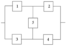Figure 2. schematic of bridge system

Objective functions and constraints of example 1 are stated as follows.

(22)

(23)

(24)

(25)

(26)

(27)

(28)

(29)

(30)

(31)

(32)

(33)

(34)

(35)

(36)

The parameters α_i and β_i are related to the physical features of system components.

Example 2 (protection system of a gas turbine)

The second example is about a series system with four subsystems that is shown in figure 3.

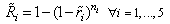
Figure 3. schematic of a series system

Objective functions and constraints of the second example are stated as follows.

(37)

(38)

(39)

(40)

(41)

(42)

(43)

(44)

(45)

(46)

(47)

(48)

(49)

(50)

(51)

(52)

(53)

The results of solving the two sample examples are shown in tables (1) and (2).

Table 1. Results of example 1 I 0.01 0.02 0.03 0.04 0.05 0.06 0.07 0.08 0.09 0.1 Number of non-dominated solutions in repository 40 45 50 36 42 47 36 31 40 38 Mean of cost (z1) 139.95 147.86 139.57 168.45 160.01 112.92 145.61 122.48 117.48 105.29 Mean of reliability (z2) 0.78 0.79 0.66 0.75 0.74 0.69 0.70 0.71 0.75 0.84 A typical solution x1 3 3 1 4 3 3 3 4 4 3 x2 1 3 2 3 4 3 2 4 4 2 x3 3 2 4 1 2 2 3 1 1 2 x4 4 2 3 1 2 3 4 1 1 4 x5 1 2 1 1 1 2 1 1 1 1 r1 0.671 0.879 0.808 0.775 0.834 0.691 0.536 0.792 0.822 0.5659 r2 0.573 0.865 0.906 0.854 0.891 0.853 0.798 0.854 0.927 0.9046 r3 0.850 0.597 0.763 0.917 0.728 0.912 0.822 0.750 0.513 0.9030 r4 0.760 0.738 0.685 0.801 0.240 0.517 0.753 0.660 0.610 0.7486 r5 0.759 0.357 0.641 0.384 0.605 0.749 0.504 0.805 0.386 0.5489 z1 145.29 174.48 141.26 153.15 154.43 141.75 151.47 0.99 0.99 0.9974 z2 0.998 0.999 0.997 0.998 0.998 0.998 0.998 157.52 169.4 174.14

Table 2. Results of example 2 I 0.01 0.02 0.03 0.04 0.05 0.06 0.07 0.08 0.09 0.1 Number of non-dominated solutions in repository 44 44 49 46 42 48 49 45 48 45 Mean of cost (z1) 163.92 84.13 167.18 96.53 80.70 68.69 48.41 61.66 158.08 67.127 Mean of reliability (z2) 0.61 0.64 0.64 0.65 0.72 0.67 0.58 0.79 0.58 0.6125 A typical solution x1 4 2 6 4 4 6 3 4 3 3 x2 5 7 6 5 5 4 7 6 5 7 x3 5 4 4 4 5 3 4 5 5 4 x4 4 5 4 4 5 6 5 5 6 5 r1 0.836 0.947 0.825 0.8692 0.885 0.744 0.969 0.880 0.911 0.969 r2 0.675 0.668 0.856 0.863 0.8583 0.860 0.656 0.000 0.939 0.777 r3 0.8241 0.913 0.849 0.892 0.834 0.989 0.896 0.949 0.918 0.920 r4 0.825 0.877 0.923 0.869 0.872 0.738 0.817 0.872 0.790 0.850 z1 105.92 265.88 379.51 248.86 279.06 353.94 270.06 319.21 288.05 397.99 z2 0.994 0.996 0.999 0.998 0.999 0.998 0.998 0.998 0.997 0.998

The examples are solved with different values of reliability interval (I). There are a lot of non-dominated solutions for each I. Therefore, in the above tables, only number of non-dominated solutions in the repository and mean of the first and second objective functions for the obtained non-dominated solutions are stated. Also for each I, one of the efficient solutions are stated. It is necessary to mention that some solutions (less than 5%) have very high costs (such as thousands and more) and are not shown in the tables. Figures (4) and (5) show non-dominated solutions for different values of I for the examples 1 and 2, respectively. (Appendix)

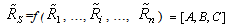
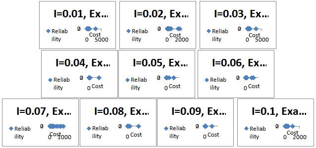Figure 5. Non-dominated solutions for example 1 for different values of I

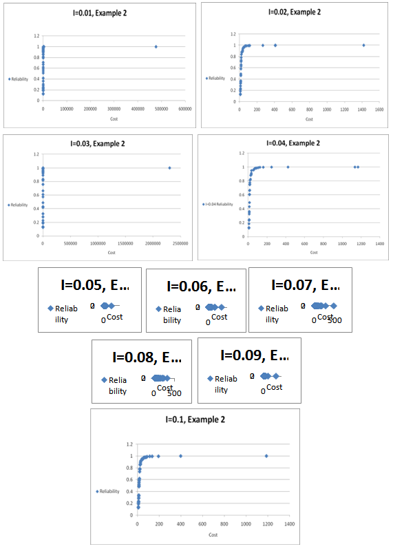Figure 6. Non-dominated solutions for example 2 for different values of I

6. Conclusions and Future Researches

In this research, multi-objective redundancy allocation problem has been investigated. The decision variables of the problem are specifying the redundancy level (number of components) and the reliability of each component in the subsystems. The research includes two major contributions to develop a novel model. The first contribution is with regards to reliability as a triangular fuzzy number, while the second examines discount rates for cost of the components in three levels. The developed fuzzy model is converted to a crisp model by using the expected value of fuzzy numbers. Then, multi-objective particle swarm optimization (MOPSO) approach is used to solve the two examples of the developed model. The results show that the proposed approach can help decision makers decide about the number of redundant components and their reliability in a subsystem to have a system that satisfies both reliability and cost criteria effectively. In other words, the obtained information from solving multi-objective model is more than single objective mode[2]. Reference[2] only presented one solution that optimized objective function and satisfied constraints. But, in this article, a set of solutions are presented that are non-dominated relative to each other. These solutions enable a decision maker (DM) to select the final alternative by his/her technical and cost preferences.

In summary, this paper presents a unique standard methodology for multi-objective redundancy allocation problem. The structure and approach of this paper could be applied for continuous assessment and improvement of RRAP with respect to reliability and cost aspects.

The research offers the following subjects for further researches: (a) applying the proposed model and procedure for multi- state systems; (b) using other meta-heuristic methods and comparing their results with those of MOPSO; (c) applying proposed approach for K-out-of-N subsystems, and, (d) considering that cost of each component depends on fuzzy parameters of reliability of that component. The reason for item (d) is that the more the tolerance of reliability is decreased, the more the component is reliable, and the more, naturally, its cost increases.

ACKNOWLEDGEMENTS

The authors would like to thank the referees for their helpful comments which significantly improved the quality of this paper. This study was supported by a grant from University of Tehran (Grant No. 27775/1/04). The authors are also grateful for the support provided by the College of Engineering, University of Tehran, Iran

Appendix

Matlab codes of multi-objective model

tic

% Example 2

y=5 %number of subsystems in system

x=2*y %number of cells in a solution. Each subsystem has two cells, one for number of components and one for reliability number

c1=2 %c1 and c2 in velocity equation

c2=2 %c1 and c2 in velocity equation

n=20 %number of particles in swarm

m=50 %number of particles in repository

ni=50 % Number of iterations (swarm)

%RLF=1 % (Redundant Lower Factor) that indicates lower limit of components in a subsystem

RUF=10 % (Redundant Upper Factor) that indicates upper limit of components in a subsystem

%RLL=0.5 % (Reliability Lower Limit) that indicates lower limit of reliability of each component

%RUL=1 % (Reliability Upper Limit) that indicates upper limit of reliability of each component

% Parameters of Example 2

Alfa=[2.33*10^(-5),1.45*10^(-5),0.541*10^(-5),8.050*10^(-5),1.950*10^(-5)]

Beta=[1.5,1.5,1.5,1.5,1.5]

v=[(1/7)^0.5,(1/4)^0.5,(3/8)^0.5,(2/3)^0.5,(2/9)^0.5]

w=[7,8,8,6,9]

V=110

C=175

W=200

T=1000

vel=zeros(n,x) % Setting initial velocity

w=0.4 % coefficient of inertia weight

swarm=zeros(n,x) % Initial Swarm of particles

ofswarm=zeros(n,2) % Matrix that contains objective function values

tempswarm=zeros(n,x) % Temporal Swarm of particles in each iteration

tempofswarm=zeros(n,2) % Matrix that contains objective function values

pbest=zeros(n,x) % Matrix that contain pbest of each particles

ofbest=zeros(n,2) % Matrix that contain objective functions of pbest solutions

rep=zeros(m,x) % Reprository

ofrep=zeros(m,2)

temprep=zeros(n+m,x) % temporal Reprository

tempofrep=zeros(n+m,2)

for i=1:n

for j=1:y

swarm(i,j)=randint(1,1,[1,RUF])

end

for j=y+1:x

swarm(i,j)=0.5+(rand/2)

end

end

% Initial population is generated

swarm=feasibleswarm1(swarm)

ofswarm=calofswarm(swarm)

iswarm=swarm % Storing initial population in memory

iofswarm=ofswarm

pbest=swarm

ofbest=ofswarm

for r=2:ni % Initial of main loop

for i=1:n

for j=1:x

temprep(i,j)=swarm(i,j)

%temprankrep(i,j)=rankswarm(i,j)

end

end

for i=n+1:n+m

for j=1:x

temprep(i,j)=rep(i-n,j)

%temprankrep(i,j)=rankrep(i-n,j)

end

end

for i=1:n

for j=1:2

tempofrep(i,j)=ofswarm(i,j)

end

end

for i=n+1:n+m

for j=1:2

tempofrep(i,j)=ofrep(i-n,j)

end

end

index=indexrep(tempofrep,n,m)

for i=1:m

t=index(i,1)

if (t>0)

rep(i,:)=temprep(t,:)

%rankrep(i,:)=temprankrep(t,:)

ofrep(i,:)=tempofrep(t,:)

end

if (t==0)

rep(i,:)=zeros(1,x)

%rankrep(i,:)=zeros(1,x)

ofrep(i,:)=zeros(1,2)

end

end

% Reporsity is updated

for i=1:n

t=index(m+1,1)

vel(i,:)=(w*vel(i,:))+(c1*rand*(pbest(i,:)-swarm(i,:)))+(c2*rand*(temprep(t,:)-swarm(i,:)))

end

for i=1:n

tempswarm(i,:)=swarm(i,:)+vel(i,:)

end

%temprankswarm=rankingswarm(tempswarm)

tempofswarm=calofswarm(tempswarm)

swarm=tempswarm

%rankswarm=temprankswarm

swarm=feasibleswarm1(swarm)

%ofswarm=tempofswarm

ofswarm=calofswarm(swarm)

for i=1:n

if (((ofswarm(i,1)pbest(i,:)=swarm(i,:)

%pbestrank(i,:)=rankswarm(i,:)

ofbest(i,:)=ofswarm(i,:)

end

if (((ofswarm(i,1)ofbest(i,2))) || ((ofswarm(i,1)>ofbest(i,1)) & (ofswarm(i,2)if (rand<0.5)

pbest(i,:)=swarm(i,:)

%pbestrank(i,:)=rankswarm(i,:)

ofbest(i,:)=ofswarm(i,:)

end

end

end

end % End of mail loop

xlswrite('rep',rep)

%xlswrite('rankrep',rankrep)

xlswrite('ofrep',ofrep)

toc

% This function calculates objective functions of swarm

function[f1]=calofswarm(swarm)

Alfa=[2.33*10^(-5),1.45*10^(-5),0.541*10^(-5),8.050*10^(-5),1.950*10^(-5)]

Beta=[1.5,1.5,1.5,1.5,1.5]

v=[(1/7)^0.5,(1/4)^0.5,(3/8)^0.5,(2/3)^0.5,(2/9)^0.5]

w=[7,8,8,6,9]

V=110

C=175

W=200

T=1000

q1=2 % First level of discount

q2=4 % Second level of discount

Co1=0.9 %First Coefficient of discount rate

Co2=0.8 %Second Coefficient of discount rate

I=0.1

% Interval of reliability in triangular fuzzy number

%swarm=[1 2 3 4 0.9 0.8 0.7 0.6]

s=size(swarm)

n=s(1,1)

x=10

y=5

%n=10

%x=8

%y=4

ofswarm=zeros(n,2)

for i=1:n

D=zeros(1,y) % Lower number of fuzzy triangular number of cost of subsystems

E=zeros(1,y) % Center number of fuzzy triangular number of cost of subsystems

F=zeros(1,y) % Upper number of fuzzy triangular number of cost of subsystems

for j=1:y

D(1,j)=(Alfa(j)*((-T/log(swarm(i,j+y)-I))^(Beta(j))))*(swarm(i,j)+exp(0.25*swarm(i,j)))

E(1,j)=(Alfa(j)*((-T/log(swarm(i,j+y)))^(Beta(j))))*(swarm(i,j)+exp(0.25*swarm(i,j)))

F(1,j)=(Alfa(j)*((-T/log(swarm(i,j+y)+I))^(Beta(j))))*(swarm(i,j)+exp(0.25*swarm(i,j)))

if (swarm(i,j)<=q1)

D(1,j)=D(1,j)

E(1,j)=E(1,j)

F(1,j)=F(1,j)

end

if ((swarm(i,j)>q1) && (swarm(i,j)<=q2))

D(1,j)=Co1*D(1,j)

E(1,j)=Co1*E(1,j)

F(1,j)=Co1*F(1,j)

end

if (swarm(i,j)>q2)

D(1,j)=Co2*D(1,j)

E(1,j)=Co2*E(1,j)

F(1,j)=Co2*F(1,j)

end

end

Ds=0 % Lower number of fuzzy triangular number of cost of system

Es=0 % Center number of fuzzy triangular number of cost of system

Fs=0 % Upper number of fuzzy triangular number of cost of system

for j=1:y

Ds=Ds+D(1,j)

end

for j=1:y

Es=Es+E(1,j)

end

for j=1:y

Fs=Fs+F(1,j)

end

ofswarm(i,1)=(Ds+(2*Es)+Fs)/4

end

% First objective function is calculated and stored

for i=1:n

A=zeros(1,y) % Lower number of fuzzy triangular number of reliability of subsystems

B=zeros(1,y) % Center number of fuzzy triangular number of reliability of subsystems

C=zeros(1,y) % Upper number of fuzzy triangular number of reliability of subsystems

for j=1:y

A(1,j)=1-((1-swarm(i,j+y)+I)^(swarm(i,j)))

B(1,j)=1-((1-swarm(i,j+y))^(swarm(i,j)))

C(1,j)=1-((1-swarm(i,j+y)-I)^(swarm(i,j)))

end

As1=0

Bs1=0

Cs1=0

As2=0

Bs2=0

Cs2=0

As=0 % Lower number of fuzzy triangular number of reliability of system

Bs=0 % Center number of fuzzy triangular number of reliability of system

Cs=0 % Upper number of fuzzy triangular number of reliability of system

As1=(A(1,1)*A(1,2))+(A(1,3)*A(1,4))+(A(1,1)*A(1,4)*A(1,5))+(A(1,2)*A(1,3)*A(1,5))+(2*A(1,1)*A(1,2)*A(1,3)*A(1,4)*A(1,5))

Bs1=(B(1,1)*B(1,2))+(B(1,3)*B(1,4))+(B(1,1)*B(1,4)*B(1,5))+(B(1,2)*B(1,3)*B(1,5))+(2*B(1,1)*B(1,2)*B(1,3)*B(1,4)*B(1,5))

Cs1=(C(1,1)*C(1,2))+(C(1,3)*C(1,4))+(C(1,1)*C(1,4)*C(1,5))+(C(1,2)*C(1,3)*C(1,5))+(2*C(1,1)*C(1,2)*C(1,3)*C(1,4)*C(1,5))

As2=(A(1,1)*A(1,2)*A(1,3)*A(1,4))+(A(1,1)*A(1,2)*A(1,3)*A(1,5))+(A(1,1)*A(1,2)*A(1,4)*A(1,5))+(A(1,1)*A(1,3)*A(1,4)*A(1,5))+(A(1,2)*A(1,3)*A(1,4)*A(1,5))

Bs2=(B(1,1)*B(1,2)*B(1,3)*B(1,4))+(B(1,1)*B(1,2)*B(1,3)*B(1,5))+(B(1,1)*B(1,2)*B(1,4)*B(1,5))+(B(1,1)*B(1,3)*B(1,4)*B(1,5))+(B(1,2)*B(1,3)*B(1,4)*B(1,5))

Cs2=(C(1,1)*C(1,2)*C(1,3)*C(1,4))+(C(1,1)*C(1,2)*C(1,3)*C(1,5))+(C(1,1)*C(1,2)*C(1,4)*C(1,5))+(C(1,1)*C(1,3)*C(1,4)*C(1,5))+(C(1,2)*C(1,3)*C(1,4)*C(1,5))

As=As1-Cs2

Bs=Bs1-Bs2

Cs=Cs1-As2

ofswarm(i,2)=(1-((As+(2*Bs)+Cs)/4))*1000

end

% Second objective function is calculated and stored

f1=ofswarm

% Constraint Handling function that converts an unfeasible solution to a feasible solution

function[f1]=feasibleswarm1(swarm)

%y=4 %number of subsystems in system

%x=2*y %number of cells in a solution. Each subsystem has two cells, one for number of components and one for reliability number

c1=2 %c1 and c2 in velocity equation

c2=2 %c1 and c2 in velocity equation

%n=10 %number of particles in swarm

m=50 %number of particles in repository

ni=50 % Number of iterations (swarm)

RLF=1 % (Redundant Lower Factor) that indicates lower limit of components in a subsystem

RUF=10 % (Redundant Upper Factor) that indicates upper limit of components in a subsystem

RLL=0 % (Reliability Lower Limit) that indicates lower limit of reliability of each component

RUL=1 % (Reliability Upper Limit) that indicates upper limit of reliability of each component

% Parameters of Example 2

Alfa=[2.33*10^(-5),1.45*10^(-5),0.541*10^(-5),8.050*10^(-5),1.950*10^(-5)]

Beta=[1.5,1.5,1.5,1.5,1.5]

v=[(1/7)^0.5,(1/4)^0.5,(3/8)^0.5,(2/3)^0.5,(2/9)^0.5]

w=[7,8,8,6,9]

V=110

C=175

W=200

T=1000

s=size(swarm)

n=s(1,1)

x=s(1,2)

y=x/2

for i=1:n

indicator=0 % Indicator that shows number of constraints that is satisfied

for j=1:y

if (ne(swarm(i,j),round(swarm(i,j)))==1)

swarm(i,j)=round(swarm(i,j))

end

end

while (indicator<((2*y)+2))

indicator=0

% Constraint of volume

SV=0 % Sum of volume

for j=1:y

SV=SV+(w(j)*(v(j)^2)*(swarm(i,j)^2))

end

if (SV<=V)

indicator=indicator+1

end

if (SV>V)

a=randint(1,1,[1,y])

if (swarm(i,a)>1)

swarm(i,a)=swarm(i,a)-1

end

end

% Constraint of weight

SW=0 % Sum of weight

for j=1:y

SW=SW+(w(j)*(swarm(i,j))*exp(0.25*swarm(i,j)))

end

if (SW<=W)

indicator=indicator+1

end

if (SW>W)

a=randint(1,1,[1,y])

if (swarm(i,a)>1)

swarm(i,a)=swarm(i,a)-1

end

end

% Constraint of number of components

for j=1:y

if ((swarm(i,j)>=RLF) && (swarm(i,j)<=RUF))

indicator=indicator+1

end

if (swarm(i,j)swarm(i,j)=RLF

end

if (swarm(i,j)>RUF)

swarm(i,j)=RUF

end

end

% Constraint of reliability of components

for j=1:y

if ((swarm(i,j+y)>=RLL) && (swarm(i,j+y)<=RUL))

indicator=indicator+1

end

if (swarm(i,j+y)swarm(i,j+y)=rand

end

if (swarm(i,j+y)>=RUL)

swarm(i,j+y)=rand

end

end

end

end

f1=swarm

function[f1]=indexrep(tempofrep,n,m)

MM=10^5 % Big number for calculating crowding distance

percent=10 % Percent of repository that is candidated for selecting H

p=n+m

M=max(max(tempofrep))+1

for i=1:p

for j=1:2

if (tempofrep(i,j)==0)

tempofrep(i,j)=M

end

end

end

dom=zeros(p,p) % Matrix that show dominance relation between solutions: If solution i dominate solution j Then dom(i,j)=1

for i=1:p

for j=1:p

if ((tempofrep(i,1)dom(i,j)=1

end

if ((tempofrep(i,1)<= tempofrep(j,1)) & (tempofrep(i,2)< tempofrep(j,2)))

dom(i,j)=1

end

if ((tempofrep(i,1)==tempofrep(j,1)) & (tempofrep(i,2)== tempofrep(j,2)) & (idom(i,j)=1

end

end

end

sum=zeros(1,p)

for j=1:p

for i=1:p

sum(1,j)=sum(1,j)+dom(i,j) %Calculating sum of columns of dom matrix

end

end

q=0

index=zeros(p,1) % Array that contains number of solutions (from p solutions) that is non dominated

for i=1:p

if (sum(1,i)==0)

q=q+1

index(q,1)=i

end

end

of=zeros(q,2) % Matrix that contains objective functions of q non dominated solutions

for i=1:q

for j=1:2

of(i,j)=tempofrep(index(i,1),j)

end

end

sortof=sort(of) % Matrix that contains sorted objective functions of q non dominated solutions

cd=zeros(q,1) % Crowding distance matrix that contains crowding distance of q non dominated solutions

for i=1:q

for j=1:2

for k=1:q

if (of(i,j)==sortof(k,j))

if ((k==1) || (k==q))

cd(i,1)=cd(i,1)+MM

else

cd(i,1)=cd(i,1)+((sortof(k+1,j)-sortof(k-1,j))/(sortof(q,j)-sortof(1,j)))

end

end

end

end

end

indexcd=zeros(q,2) % Matrix that contains both index and cd matrixes

for i=1:q

indexcd(i,1)=index(i,1)

indexcd(i,2)=cd(i,1)

end

indexcd=sortrows(indexcd,2)

for i=1:q

indexcd2(i,1)=indexcd(q+1-i,1)

indexcd2(i,2)=indexcd(q+1-i,2)

end

indexcd=indexcd2

index=indexcd(:,1)

indexrep=zeros(m+1,1) %Matrix that contain indices of m repository solutions and H index that is selected from repository

if (q>=m)

for i=1:m

indexrep(i,1)=index(i,1)

end

else

for i=1:q

indexrep(i,1)=index(i,1)

end

for i=q+1:m

indexrep(i,1)=0

end

end

z=ceil((m*percent)/100)

flag=0

while (flag==0)

H=randint(1,1,[1,z])

if (H<=q)

flag=1

end

end

indexrep(m+1,1)=index(H,1)

f1=indexrep

indexrep

q