-
Paper Information
- Paper Submission
-
Journal Information
- About This Journal
- Editorial Board
- Current Issue
- Archive
- Author Guidelines
- Contact Us
Resources and Environment
p-ISSN: 2163-2618 e-ISSN: 2163-2634
2024; 14(2): 33-44
doi:10.5923/j.re.20241402.01
Received: Jun. 1, 2024; Accepted: Jun. 19, 2024; Published: Jun. 22, 2024

Extreme Precipitation in Madagascar Part II: Establishing Frequency Isohyets by Spatial Interpolation (Kriging)
 Abstract
 Reference
 Full-Text PDF
 Full-text HTML
Justin Ratsaramody
Laboratoire d'Hydraulique, Ecole Supérieure Polytechnique, Université d'Antsiranana, Madagascar
Correspondence to: Justin Ratsaramody, Laboratoire d'Hydraulique, Ecole Supérieure Polytechnique, Université d'Antsiranana, Madagascar.
| Email: |  |
Copyright © 2024 The Author(s). Published by Scientific & Academic Publishing.
This work is licensed under the Creative Commons Attribution International License (CC BY).
http://creativecommons.org/licenses/by/4.0/

In this second part of the studies on extreme rainfall in Madagascar, the central question is that of spatial interpola-tion in order to produce isohyet maps corresponding to different return periods with processing the series of maximum annual daily rainfall from 1970 to 2023 across 132 observed sites. The results showed that, contrary to traditional practice in Madagascar, the data from all the sites could not be modelled solely by a Gumbel distribution but that a significant proportion (28.7%) had to be modelled by a GEV distribution to take account of climate change. The results also showed the presence of a spatial trend in the form of an affine surface that had to be removed before any spatial interpolation. Normalization with the Box-Cox transformation of the raw data was made necessary by the non-stationary nature of the raw data. There is geometric anisotropy in the data, but this had no significant influence on the spatial interpolation results. Compared through cross-validation and diagnostic metrics, it was found that the Ordinary Kriging interpolation model was better than Universal Kriging even though the variances of the prediction residuals of these two models were almost identical. Cross-validation showed that the two models both overestimated predictions beyond a threshold value, but that these deviations were negligible. The spatial interpolation results obtained from this work using Ordinary Kriging, which was then used to draw the frequency isohyet maps, are extremely accurate because the variances are of the order of a millimetre and these differences are generally outside the Madagascar area.
Keywords: Spatial structure, Trend surfaces, Box-Cox, Ordinary Kriging, Universal Kriging, Frequency isohyets
Cite this paper: Justin Ratsaramody, Extreme Precipitation in Madagascar Part II: Establishing Frequency Isohyets by Spatial Interpolation (Kriging), Resources and Environment, Vol. 14 No. 2, 2024, pp. 33-44. doi: 10.5923/j.re.20241402.01.
Article Outline
1. Introduction
- In the first part of this series of two articles [1], the process of frequency analysis of extreme daily maximum rainfall data for Madagascar using the Block Maxima method was studied for the 1970-2023 and 2000-2023 time series, and the results for the six provincial capitals were presented as an example. In particular, these results showed that stationary GEV models produced unrealistic results and that the return periods for the same extreme event were different because they depended on the size of the time series considered. In addition, despite the fact that the two time series were nested, it was also found that the trends, reflecting climate change, were different and even in the opposite direction in some cases. For better statistical modelling, the longest series (1970-2023) had then been studied and, to take account of climate change, non-stationary GEV distribution models were applied to this time series with variation as a function of time of the position parameter
 and the scale parameter
  but keeping the shape parameter
  constant. This resulted in eight possible non-stationary models depending on the values of the intercepts
  and
and  and the values of the slopes
  and
and  . These models also included the special case of the Gumbel distribution when the slopes were zero, i.e.
  and
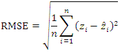
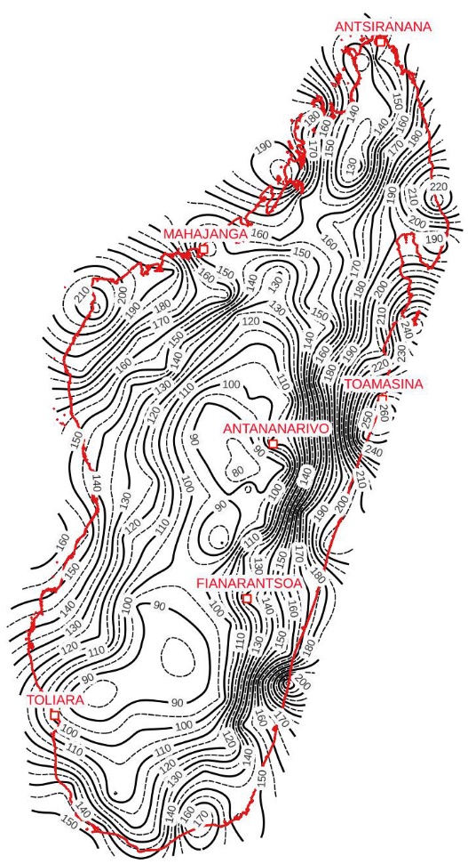
and  . This led to much more realistic results, but in which the one-to-one relationship between the return period and the return level was called into question by the presence of a third parameter interpreted as the risk level. Even if this process of frequency analysis were absolutely necessary to determine the return period and/or the return level at a given spatial point, it is extremely cumbersome and tedious and may not be within everyone's reach, particularly for engineers in charge of establishing design flows for hydraulic and road infrastructures, etc. In this case, a map of frequency isohyets is much more practical because, for a return period and an estimated level of risk, all you have to do is identify the spatial point concerned on the map and read the value of the corresponding return period. This would considerably reduce the time spent on this activity in projects and studies in various fields such as flood risk assessment and mitigation, environmental impact studies, land-use planning, river restoration and the design of hydraulic structures, etc. [2]. Such maps are produced using spatial interpolation methods because of the presence of ungauged areas, which is the case for virtually all of Madagascar, and the entire frequency analysis process described above was carried out beforehand on the 132 measurement points shown in Figure 1. These points were chosen at random but so that there was at least 1 measurement point in all 119 districts of Madagascar.
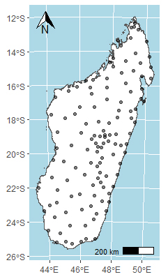 | Figure 1. Locations of rainfall data sites on the island of Madagascar |
2. Materials
2.1. Rainfall Data
- The rainfall data are those used in the first article, i.e. daily rainfall data from 1970 to 2023, combined with GLDAS (1970 to 2000), TRMM (2001 to 2019) and GPM (2020 to 2023) data. They were obtained from gridded data, but reduced to the measurement points (Figure 1) and downloaded from the https://giovanni.gsfc.nasa.gov/website.
2.2. Digital Elevation Model (DEM)
- The DEM used for this study was a set of DEMs produced by SRTM (Shuttle Radar Topography Mission) and available at https://earthexplorer.usgs.gov/. After being assembled, the various tiles were projected onto the CSR EPSG: 29702, which is the CSR covering the entire island of Madagascar.
2.3. Spatial Interpolation Grid
- The spatial interpolation grid used for this study was a grid with square cells of dimensions 5000 m × 5000 m, which provides sufficient accuracy given the large size of the country (1700 km × 500 km) while maintaining a certain fluidity in the calculations.
2.4. Calculation Tools
- All calculations relating to this study were carried out using the free software R 4.3.2 (https://www.r-project.org/ ) with the corresponding packages, mainly the gstat package [19] and its dependencies. Other packages were also used for the various operations required.
3. Methodology
3.1. Preliminary Analysis
- In order to determine the return levels corresponding to the different return periods
 = 10, 20, 50, 100 and 200 years, the entire procedure described in the first article was applied to each of the 132 measurement points shown in Figure 1 with non-stationary GEV distribution models.
3.2. Exploratory Analysis and Spatial Structure of the Data
- In this analysis, the aim was to examine both the statistical distribution of the various values of
 (24-hour rainfall with a return period of
  years) and the spatial distribution of these values in order to detect a spatial trend. Indeed, as we propose to carry out an interpolation by kriging, this is only possible if the process that generated the values at the observation points is a random process following a normal distribution and if, spatially, they have a stationary structure (Gaussian fields) [10]. To verify the normality of the data, summary statistics were calculated to account for the asymmetry and dispersion of the data. The presence of a spatial trend was also highlighted using a map of observed points weighted by their values, as well as the polynomial regression of
  values against X and Y coordinates.
3.3. Normalisation of the Data
- For geostatistical modelling to be possible, the data must be (approximately) normally distributed and stationary, i.e. the mean and variance must not vary significantly in space. To make the
 of
of  approximate to a normal distribution, the well-known Box-Cox transformation was used [20,21]:
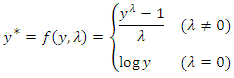 | (1) |
 , which follows a normal distribution. The parameter
  was determined using the maximum likelihood (ML) method. These transformed
  data were then used for spatial interpolation. To return to the initial data
  the inverse transformations are immediate by inverting equations (1):
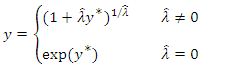 | (2) |
 is the estimated value of the parameter
  .
.3.4. Spatial Interpolation
- Generally speaking and whatever the method used, the objective of spatial interpolation is to determine the value
 at a non-gauged location,
  knowing the values at
  locations
  where
where  is a location and
  and
and  are the coordinates in geographical space. Thus, at an ungauged point
  this value
  is given by
  | (3) |
 is the weight for gauged station
  However, as already indicated above, the spatial interpolation considered in this study is spatial interpolation by kriging, despite the fact that there are other forms of spatial interpolation, such as the very popular IDW [12,22], which we did not use because of the subjectivity involved in choosing the power parameter to be applied to the inverse distance. The kriging interpolation method differs in that it provides an unbiased estimate by considering the autocorrelation of all available data on the basis of various semivariograms [23].
3.4.1. Empirical Semivariogram
- Under the assumption of intrinsic stationarity, it is assumed that the process which generated the samples at the measured points
 is a random function
  composed of a mean
  and a residual
  [24,25]:
 | (4) |
 | (5) |
 is constant and the spatial correlation of
  does not depend on the location
  but only on the separation distance
  It is then possible to form several pairs
  whose separation vectors
  are (almost) identical and estimate the correlation from these. The empirical semivariogram obtained from the transformed data
  in equation (1) is then defined according to equation (6):
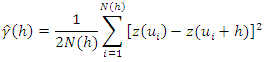 | (6) |
 is the measured semivariance for distance
  is the number of data pairs separated by distance
  and
and  is the value of the variable at location
  In addition to what has been done in the exploratory analysis, the empirical semivariogram is a valuable exploratory tool for assessing the presence of spatial correlation in the data. It should also be noted that, under the assumption of intrinsic second-order stationarity, the empirical semivariogram expressed by equation (6) is an unbiased estimator of the theoretical semivariogram expressed by equation (7) below because the unknown mean of the random function is not involved in the expression of the empirical semivariogram in equation (6).
3.4.2. Theoretical Semivariogram Models
- As the empirical semivariogram only covers the observed points, it has to be adjusted by a theoretical model to cover the entire space of points to be interpolated. Under the assumption of second-order stationarity and the intrinsic assumption, the semivariogram shows how the dissimilarity between
 and
and  changes with distance
  [26]:
[26]: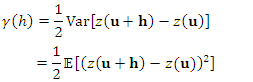 | (7) |
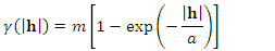 | (8) |
 is the value of the semivariogram when it reaches the sill, and
  is the range. For this model, the practical range
  is defined as the distance for which
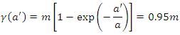 | (9) |
 • the spherical model:
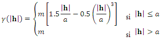 | (10) |
 and the range
  .• the Gaussian model:
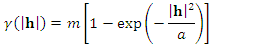 | (11) |
 and the range
  .
.3.4.3. Anisotropy
- When the theoretical models given by equations (5), (7) and (8) are isotropic, the overall omnidirectional semivariogram depends only on the length of vector
 , i.e.
 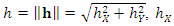 and
and  being the components of vector
  projected onto X and Y. However, anisotropy has an important effect on kriging weights because, if it exists, the weight of points located in the main direction of the anisotropy ellipse will increase: it is therefore essential to analyse the presence of anisotropy in the data. When geometric anisotropy exists in the stationary case, it implies that the thresholds of the directional semivariograms, although equal, are reached with two different distances (ranges). The anisotropy ratio is defined as follows [12]:
 | (12) |
 is the largest range in the direction of the major axis and
  is the smallest span in the direction of the minor axis. The spatial variation between any pair
  and
and  is then calculated by the distance
  in the maximum continuity axis variogram model according to the rotation angle
  and the anisotropy ratio
  where
where  is given by equation (11) below [12,27]:
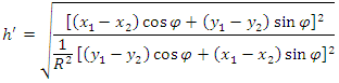 | (13) |
 the omnidirectional empirical semivariogram
  will then be used to be fitted by the best of one of the theoretical models (equations (7), (9) and (10)) for kriging interpolation.
3.4.4. Ordinary Kriging
- We have Ordinary Kriging (OK) when, in equation (4) above, the mean m is constant (or zero) and the kriging is then done on the residuals
 . For Ordinary Kriging (OK), the weights
  in equation (3) are obtained by solving the following system of linear equations [12,28]:
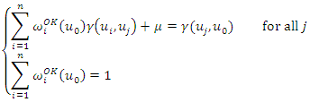 | (14) |
 is the value of the theoretical semivariogram function for the distance between
  and
and  is the value of the theoretical semivariogram of the distance between
  and
and  is the Lagrange parameter. The second equation in (14) ensures that the interpolation is unbiased.
3.4.5. Universal Kriging (UK)
- When, in equation (4), the mean m of the measured data is no longer stationary but depends on the X and Y coordinates, this confirms the presence of a trend that needs to be removed, and interpolation then needs to be performed on the remaining residuals. Interpolation by kriging can only be performed on random fields that are substantially Gaussian [10]. The predictions
 at the ungauged locations
  are then obtained from:
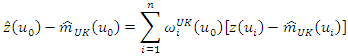 | (15) |
 replaced by
  from equation (15). As for the mean
  which includes the spatial tendency to be removed, it is generally expressed in the form of a first or second degree polynomial [25,29]:
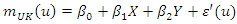 | (16) |
 | (17) |
 are regression coefficients to be determined and
  are regression residuals. In the case of equation (16), the trend surface is an affine surface while in the case of equation (17), the trend surface is a quadratic surface.
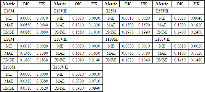
3.5. Assessment of Model Quality
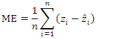
- Given the large amount of modelling to be carried out in this work, it was necessary to have criteria and/or procedures for evaluating the quality of these models in order to choose the best model. The performance of the final theoretical semivariogram model, and hence of the kriging predictions, is assessed using leave-one-out cross-validation [30], a procedure in which the observed values of the data are eliminated one by one and then predictions are made for each of these data using the remaining data [31,32]. The predicted values are then compared with the observed values.The quality of the interpolation fit was also assessed by comparing the following diagnostic metrics [22,33,34]: the mean error ME, which measures bias, the mean absolute error MAE and the root mean square error RMSE:
 | (18) |
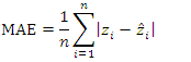 | (19) |
 | (20) |
 and
and  are the observed and predicted values, respectively, at the same point
  is the number of observation points. The closer the values of ME, MAE and RMSE are to zero, the better the fit.
4. Results and Discussion
- As already indicated, the results shown in the figures are for the 10-year return period T10VH (Very High), but the tables show all the results.
4.1. Results of the Preliminary Analysis
- In a non-stationary context and after applying the procedures described in the first article for the 1970-2023 series of annual maxima, the distributions found for the 132 data points are shown in Figure 2. For the GEV distributions, the shape coefficient was such that
 while for the Gumbel distributions, we had
  for this shape coefficient.Traditionally, the Gumbel distribution had always been the distribution used in Madagascar. However, the results show that this is not entirely correct, since 28.7% of the measurement points here follow a GEV distribution, even though the vast majority (71.3%) follow a Gumbel distribution. Figure 2 also shows that there is no preferred location for the nature of the distribution (GEV or Gumbel) either in relation to coastal areas or in relation to elevation.
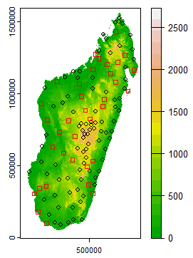 | Figure 2. Distribution models on a terrain relief background (elevation in metres). Black circles: Gumbel model (87), red squares: GEV model (35) |
4.2. Results of the Exploratory Analysis and the Spatial Structure of the Data
- The skewness coefficients for the data leading to the 10 maps considered are shown in Table 1.
|
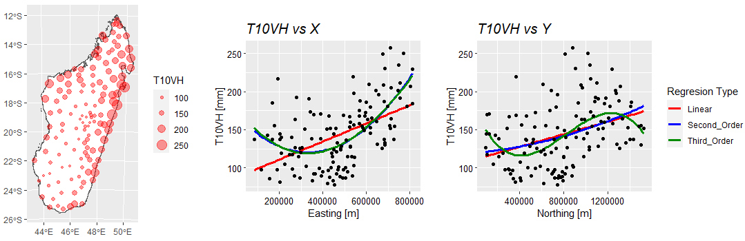 | Figure 3. Left: Map of proportional values of T10VH. Right: Polynomial regressions of T10VH as a function of X and Y coordinates |
4.3. Results of Trend Surface Calculations
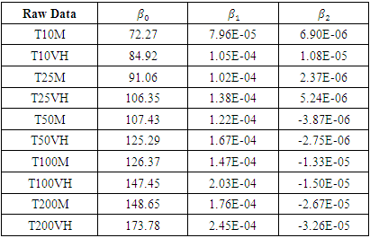
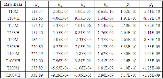
- As the presence of a trend was highlighted above in Section 4.2, it is important to confirm its existence in the data. Note that if the raw data contains a trend, the same will also be true for the Box-Cox transformed data (BC data). The
 parameters of the trend surface equations (16) and (17) had been determined by ordinary least squares and are shown in Tables 2 and 3.
|
|
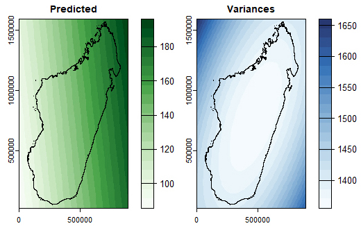 | Figure 4. Map of the trend surface predicted by the 1st order model and map of the variances of its residuals (T10VH) |
 | Figure 5. Map of the trend surface predicted by the 2nd order model and map of the variances of its residuals (T10VH) |
 coefficients,
  to 5, of the second-order terms are all less than 10-9 for the second-order surface. This decision is consistent with the principle of parsimony in statistical modelling.Visually, if we refer to Figures 4 and 5, we can see that the high variances are found outside the island, which is normal since these are non-sampled areas.
4.4. Results of Data Normalisation
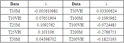
- Given the results in Table 1, a Box-Cox transformation was used to normalise the data according to equations (1) and the λ values found are summarised in Table 4.
|
4.5. Anisotropy Study Results
- As it is on the BC transformed data that the kriging interpolations will be applied, the examination of the anisotropy was carried out on this BC transformed data. The directional empirical semivariograms for T10VH and for the four main directions in space, 0, 45, 90 and 135 degrees, are shown in Figure 6.
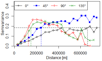 | Figure 6. Directional empirical semivariograms of BC data for T10VH. The dotted horizontal line corresponds to the sill (variance) of the BC data |
|
 , the distance
  to be considered between any pair
  and
and  in semivariogram calculations should be:
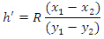 | (21) |
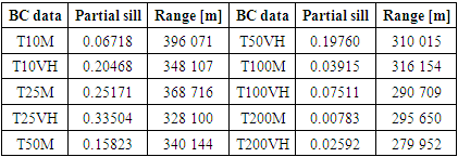
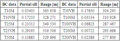
4.6. Results of Theoretical Semivariogram Models
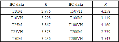
- After removing the 1st order trend, by comparing the sums of squared errors, the fits of the theoretical models to the omnidirectional semivariograms of the BC data all gave as the best model a spherical model with a zero nugget among the theoretical models tested (exponential, Gaussian and spherical). The characteristics of these models are shown in Table 6 for Ordinary Kriging and Table 7 for Universal Kriging.
|
|
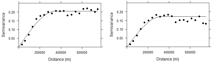 | Figure 7. Empirical semivariograms and fitted theoretical model for BC T10VH data. Left: Ordinary Kriging. Right: Universal Kriging |
4.7. OK and UK Results
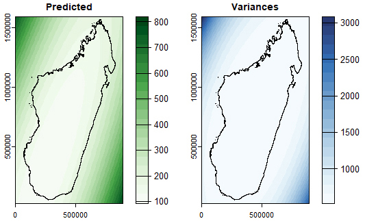
- The theoretical semivariogram models found in Section 4.6 had been applied for Ordinary Kriging (OK) and Universal Kriging (UK) on the interpolation grid described in Section 2.3 (5000 m × 5000 m). For both Ordinary Kriging and Universal Kriging, this interpolation was carried out on the residuals of the BC data and, for Universal Kriging, the trend surface (affine) was directly taken into account in the model in the form
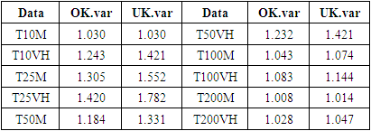
 ∼ X + Y and the interpolation was carried out on the residuals of this model.For both Ordinary Kriging and Universal Kriging, it can be seen that the variances of the prediction residuals are minimal at the observed points, which clearly confirms the unbiased nature of spatial interpolation by kriging. Furthermore, the maximum values of these variances are found outside the island of Madagascar, which is normal since these are unsampled areas.With the exception of the values, the mapping for the other data in the study shows similar patterns to Figures 8 and 9 and, to summarise, the maximum variances of these predictions are given in Table 8.
|
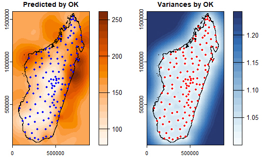 | Figure 8. Ordinary Kriging for T10VH. Left: predicted values. Right: variances of predicted residuals |
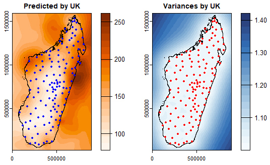 | Figure 9. Universal Kriging for T10VH. Left: predicted values. Right: variances of predicted residuals |
4.8. Quality Assessment of the Two Kriging Models
- Using the leave-one-out cross-validation (LOOCV) method, the two kriging models were compared: this method compares the predicted values with the observed values and the conclusions on the variances are similar to those obtained for Table 8 above, i.e. Ordinary Kriging presented the lowest variances at the observed points. In relation to the observed points, the two kriging models show exactly the same prediction behaviour, as shown for example in Figure 10 for the T10VH data.
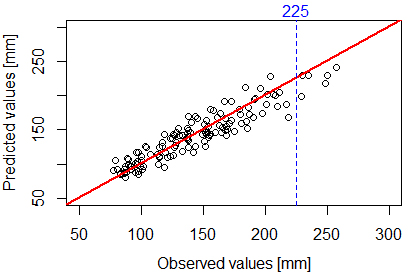 | Figure 10. Prediction behaviour of OK and UK models compared with observed values. Red line: model |
|
|
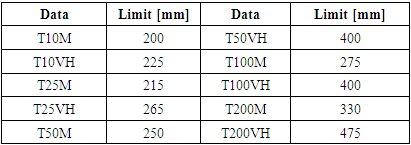
4.9. Frequency Isohyet Plot
- Based on the rasters produced by Ordinary Kriging, the frequency isohyet maps, i.e. the contour lines, were drawn using the free software QGIS. A simplified version of these maps for the T10VH data is shown in Figure 11.
 | Figure 11. Overview of the T10VH frequency isohyet map |
5. Conclusions
- This work on extreme rainfall in Madagascar consists of two articles, the final objective of which was to update the frequency isohyet maps, the most recent of which dates back to 1993. The first article dealt mainly with frequency analysis, which led to a completely different view of the notion of return period, with non-stationary models to take account of the effects of climate change.In this second article, the focus was on spatial interpolation, where a preliminary analysis of the data had shown that the traditional use of the Gumbel distribution to model extreme annual daily rainfall no longer made sense when the effects of climate change were taken into account. Analysis of the spatial structure had also shown the presence of spatial trends in the data, trends modelled by an affine surface or a quadratic surface depending on the coordinates. However, the various tests showed that this trend was best expressed by an affine surface, which was also in line with the principle of parsimony in statistical modelling.Spatial interpolation was then carried out on the Box-Cox transformed data, as the raw data showed non-negligible skewness coefficients, and two competing spatial interpolation models were considered: Ordinary Kriging and Universal Kriging. To carry out this geostatistical interpolation, after removing the trend, the directional and omnidirectional empirical semivariograms were analysed and it was shown that, despite the presence of geometric anisotropy, this had no significant influence on the interpolation results. Finally, the best theoretical models fitted to the omnidirectional semivariograms were all spherical models without nuggets, for both Ordinary Kriging and Universal Kriging.After comparing the variances of the interpolation residuals, leave-one-out cross-validation (LOOCV) and diagnostic metrics, it was found that Ordinary Kriging was better than Universal Kriging and that the final frequency isohyet maps were drawn using the rasters produced by Ordinary Kriging. The cross-validation also showed that the interpolation models found overestimated the predicted values beyond a threshold value, although the deviations were extremely small and outside the area of interest, i.e. outside Madagascar.In view of recent disasters in various fields (floods, bridge and road failures, etc.), we hope that this work will help to mitigate or even eliminate these disasters by taking into account the correct return levels and/or return periods to be applied in the design of infrastructures or in the management of areas at risk.