1. Introduction

Since the publication of the first IPCC (Intergovernmental Panel on Climate Change) report in 1993, many studies have been carried out on the global hydrological cycle [1] and climate model projections have predicted an increase in extreme precipitation events almost everywhere on the planet (for example, [2-3]). It was also shown that the increase in extreme events played a major role in the increase in total annual precipitation [4].

Madagascar is no exception to this global trend. Indeed, because of its position in the south-western basin of the Indian Ocean, the island of Madagascar is at the end of the path of cyclones that form in the eastern part of this ocean, making it a prime target. It has also been noted that over the last two decades, more and more cyclones have also been originating from the west of Madagascar, in the Mozambique Channel, and these cyclones have been just as devastating as those originating in the Indian Ocean in areas that were previously relatively spared. The rains and winds brought by these meteors have increased in intensity, causing a great deal of damage and loss of life. According to a 2016 World Bank report [5], over the period 2000-2015 alone, the passage of these meteors and the floods that followed caused almost USD 4.159 billion in damage and 1,651 deaths, not to mention the more than 2.5 million people affected and made homeless during this period.

Of the various types of damage caused by cyclones, the first is to road infrastructure, the impact of which is catastrophic for already poor populations. When roads are cut off, inflation rises immediately [5], not to mention the delays and cost of reconstruction. The Madagascar Roads Authority (ARM: Autorité Routière de Madagascar) spent €9.6 million just to repair national roads, and only for 2 cyclones in 2012: Giovanna (February 2012) and Irina (March 2012) [6]. In addition to these road infrastructures, other production infrastructures such as hydro-agricultural dams, canals and irrigation works have also been destroyed, resulting in economic losses for the population, 85% of whom are farmers in Madagascar.

Much of this damage could have been avoided if the infrastructures had been built with a design flow that took into account the return period flows corresponding to the purpose of the structures. However, the virtual absence of flow data makes this task impossible. This is why we have to turn to rainfall, which is a little more abundantly available. Subsequently, knowing the value of a maximum rainfall of 24H and return period , a design flow can be estimated using a runoff-flow model, i.e., for example, determining a maximum discharge of the same return period using a formula for calculating the maximum intensity corresponding to the characteristics of the catchment concerned (e.g., Rational Method). Presenting this maximum rainfall for a given return period in the form of a map makes the task even easier, because all you have to do is read the frequency isohyet on the map that passes through the target site (or do a little interpolation if the target site is located between two isohyets). This would significantly reduce the time it would take to estimate design rainfall in ungauged areas, with many applications such as flood risk assessment and mitigation, environmental impact assessments, land use planning, river restoration and hydraulic structure design, etc.

The present study is part of an attempt to update this type of isohyet globally, with the most recent values for the whole of Madagascar dating from 1993 [7]. Indeed, with the climate change that has occurred in recent decades, this update seemed more than necessary. In addition, the extensive research carried out in this field has led to the development of new methods, the implementation of which is facilitated by various numerical technologies that are now widely available. The present article is the first in a series of two dealing essentially with return periods and return levels with non-stationary models, while the second article concerns the development of frequency isohyets themselves.

Recently, many researchers have already pointed out the need to use non-stationary models to calculate return periods, particularly if we want to take climate change into account [8-15]. Indeed, in the context of climate change, comparative studies carried out by various researchers have shown that non-stationary distributions outperform stationary distributions [16-19].

Another problem that arises when studying extreme rainfall is the size of the time series to be used to obtain reliable estimates [1,20]. In fact, since time immemorial, at least in Madagascar, a certain value with a single return period has always been assigned to a given extreme rainfall event and vice versa, i.e. derived from stationary models. But this approach is questionable because, as will be shown below, the use of stationary models gives completely different return periods for the same rainfall depending on the size of the sample treated. However, it is difficult to know what length of series to use to obtain reliable results. All we know is that, logically, the longer the series, the better the statistical modelling should be. In this article, we use two overlapping time series, 1970-2023 (54 years) and 2000-2023 (24 years), to show that the trends are completely different depending on which series is considered.

In the entire study, 132 points were used to measure maximum annual rainfall, but due to lack of space, only the study and results for 6 measuring points corresponding to the six provincial capitals of Madagascar are presented in this article (Figure 1).

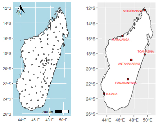Figure 1. Left: Location of the 132 measurement points. Right: the six provincial capitals

2. Materials

2.1. Rainfall Data

Given the scarcity of data covering the whole of Madagascar and available over a long period, we used gridded daily rainfall data downloaded from the website. To compile daily precipitation data from 1970 to 2023, we used GLDAS (1970 to 2000), TRMM (2001 to 2019) and GPM (2020 to 2023) data.

The sites concerned were distributed almost randomly, with at least 1 site in each of the island's 119 districts (Figure 1). For the analysis in this article, the following daily rainfall series were considered: 1970 to 2023 (n = 54 years) and 2000 to 2023 (n = 24 years).

2.2. Calculation Tools

All the calculations for this study were carried out using the free software R 4.3.2 ( ) with the corresponding packages, in particular the extRemes package [21] and its dependencies.

3. Methodology

3.1. Preliminary Analyses

As a preliminary analysis, the maximum daily precipitation was determined for each of the two series of annual precipitation maxima (1970-2023 and 2000-2023). The homogeneity of these two series was then assessed using the Mann-Whitney test. Finally, trends were identified using the Mann-Kendall test [12], while Pettitt's non-parametric algorithm [22] was used to determine the year of the trend break. For each of these three tests, the p-value at the 5% level was used to determine the results. A linear regression was also calculated for each of these two series.

Where there is an absence of homogeneity or where the presence of a trend is confirmed, this constitutes a valid hypothesis for introducing non-stationarity into the estimation [12,23].

3.2. Extreme Value Distributions

The frequency analysis of extreme maximum values is based on the Fisher-Tippet Theorem (1928), which states that the distribution of maxima, suitably normalised, behaves in the limit as a Generalized Extreme Value (GEV) distribution, independently of the distribution from which the sample data comes. The family of models of the GEV distribution can be written as [24,25]:

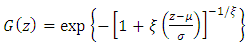(1)

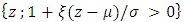defined on the set and where the parameters satisfy 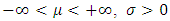and and are the location parameter, the scale parameter and the shape parameter, respectively.

The GEV distribution leads to the special cases of a Fréchet distribution a Weibull distribution and a Gumbel distribution The latter case is in fact the limit of the GEV distribution when in which case [24,25]:

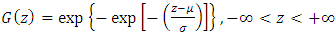(2)

It should be noted that the POT (Peak Over Threshold) method was not chosen for this study because of the need for a hypothesis that could be subjective in order to assess the threshold to be applied. Consequently, the BM (Blocks Maxima) method was used in this study. This method is widely used in the literature and has given excellent results [26]. To determine the distribution model (GEV or Gumbel) and therefore the three parameters and , the Maximum Likelihood Estimation (MLE) method had been used.

It is worth remembering that thanks to the inference of the shape parameter , it is the data itself that determines the type of distribution (Fréchet, Gumbel or Weibull) and that it is not necessary to fix the family of distributions a priori [27].

3.3. Determination of Quantiles Corresponding to Return Levels

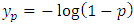
The return level expected to be exceeded on average once during the return period years, distinguishing the GEV distribution from the Gumbel distribution, is given by [24]:

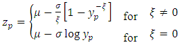(3)

with . This return period is the value of the daily rainfall with a return period that is assigned to each of the sites in the area of interest.

3.4. Stationary Models

For each of the two series, the above distribution models (equations (1) and (2)) had been applied in the stationary case i.e. assuming that the parameters and are all constant.

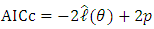(4)

where is the maximised value of the log-likelihood for a model containing parameters.

3.5. Non-Stationary Models

The stationarity assumption that data are independent and identically distributed with constant properties over time does not correspond to the variations induced by climate change. Indeed, it has been widely demonstrated that natural climate variability or variability due to anthropogenic causes mean that extreme hydroclimatic series are not stationary but vary over time [29-31,15].

In most studies of non-stationary extreme value models in the literature, the distribution models are still the GEV (equation (1)) or Gumbel (equation (2)) models but it is the parameters and that are no longer constant but are variable as a function of time and possibly other covariates [24]. However, to account for variability and trends in extreme values, it is customary to formulate the location parameter and the scale parameter as a function of time while keeping the shape parameter constant (e.g. [32,17,18,12,15]. Also in most cases, the location and scale parameters are formulated as a linear function of time according to:

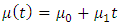(5)

(6)

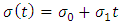
where and are parameters to be determined by regression.

Polynomial models with higher degrees could have been used, but it has been shown that such models exhibit excessive fluctuations and the forecasts obtained are highly inaccurate [33].

The computations of these non-stationary models were carried out with the extRemes R package and the authors of this package [21] recommend introducing the time covariate in the following standardised form:

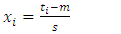(7)

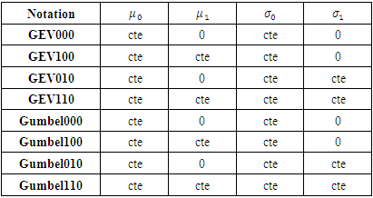
where and are respectively the mean and standard deviation of the time covariate.

Eight possible models were determined by combining the values of and In all these models, the interception parameters and only the slope parameters and change. Table 1 gives the notations that will be used for the results.

Table 1. Names of non-stationary models

For more effective statistical modelling, and therefore with a maximum sample size, only the 1970-2023 series (n = 54 years) was considered for the non-stationary models. And as with the stationary models, the best model for a given city was chosen on the basis of the AIC criterion.

3.6. Return Levels for Non-Stationary Models

Once the non-stationary model was established, the return levels were calculated with equations (3) but as the parameters and are time-varying, the return levels should also normally be time-varying. As this does not make practical sense, a second probability level has been introduced for each calculated return level. This probability level can be regarded as the risk level for the return period under consideration.

4. Results and Discussion

4.1. Maximum Daily Rainfall 1970-2023

By simple inspection, Figure 2 shows the maximum annual 24H rainfall for each of the cities studied.

Figure 2 shows that the peaks all occurred after the year 2000, i.e. in the second half of the period under consideration. The cases of Antsiranana and Antananarivo deserve particular attention in that the peaks occurred almost at the end of a period of more than 50 years. This is certainly linked to the recent environmental degradation of the regions in which these two towns are located, but further studies are needed to confirm this.

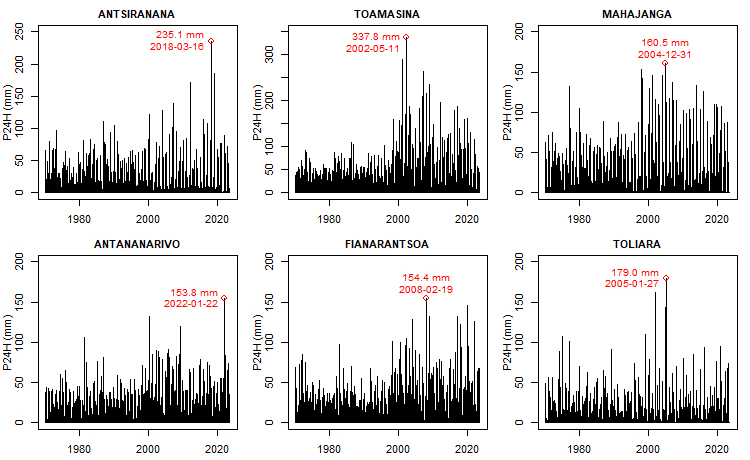Figure 2. Maximum annual rainfall series 1970-2023 with marking of maximum events and date of occurrence

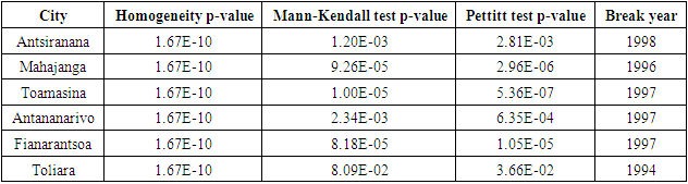
4.2. Results of Tests for Homogeneity, Trends and Break Year

For the 1970-2023 series, the results of homogeneity tests (Mann-Whitney test) and trend tests (Mann-Kendall test) as well as Pettitt tests for the presence of a break year are shown in Table 2.

Table 2. p-values of homogeneity tests, trend tests and break year (1970-2023)

At the 5% significance level, the p-values in Table 2 show that the 1970-2023 annual maximum precipitation series for each of the cities considered are non-homogeneous, all show a trend and have a break year given in the last column of Table 2. This break year also confirms the results for the date of appearance of the maximum (all after the year 2000).

Figures 3 shows these trends and a linear fit for the 1970-2023 and 2000-2023 series for the six cities studied. In these figures, blue line is a linear regression while red line is a local polynomial adjustment (loess).

Figures 3 shows that only Antsiranana shows an increasing linear trend for both the 1970-2023 and 2000-2023 series. For Fianarantsoa, the trend is upwards when considering the 1970-2023 series, and this trend is practically constant when considering the 2000-2023 series. For the other remaining cities (Mahajanga, Toamasina, Antananarivo and Toliara), the trend is upward for the 1970-2023 series, but is completely reversed when the 2000-2023 series is considered.

These changes in trend can also be explained by the fact that the 2000-2023 series occurs after the break year (Table 2). These few examples demonstrate the importance of the time series studied in relation to climate change, which can lead to very different results.

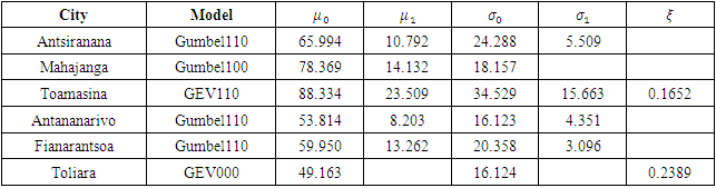
4.3. Stationary Model Results

For the cities concerned, the best stationary models with their respective parameters are shown in Table 3.

Table 3. Best models and parameters obtained for stationary cases

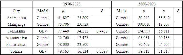
Table 3 shows that for the 2000-2023 series, all the best models are Gumbel models while for the 1970-2023 series, two series resulted in a GEV distribution The small number of cases (six in this case) does not allow us to jump to the conclusion that the shorter the series, the more the shape parameter tends towards zero. Moreover, four of the six cases in the long series 1970-2023 also gave a Gumbel distribution.

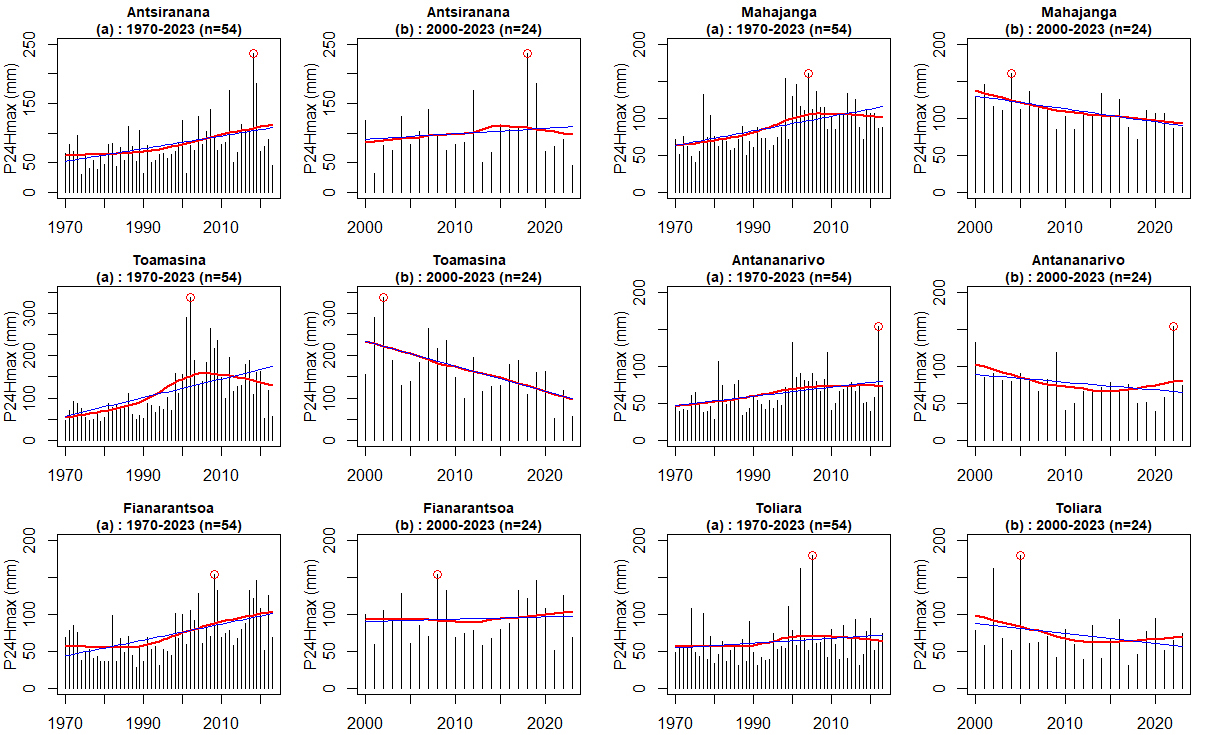Figure 3. Comparison of trends for the 1970-2023 and 2000-2023 series for provincial capitals

With regard to the return levels corresponding to different return periods, Table 4 gives the values found after applying equations (3).

Table 4. Return levels for different return periods as a function of the series studied (stationary cases)

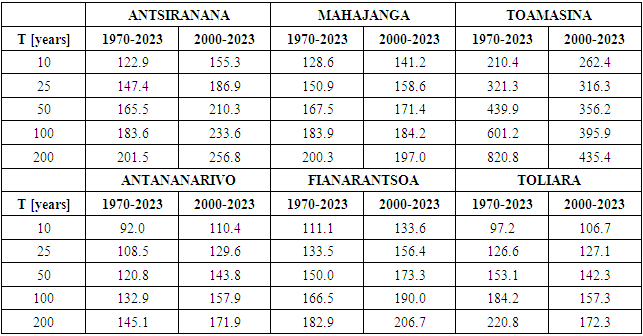
Table 4 shows that the return periods for the 2000-2023 series (the shortest) are higher than those for the 1970-2023 series (the longest) for cities with the best Gumbel distribution (see also Table 3). However, the situation is reversed for the GEV models (Toamasina and Toliara for 1970-2023) from high return periods ( years) onwards.

The results in Table 4 are more clearly visible when plotted on a graph (Figure 4).

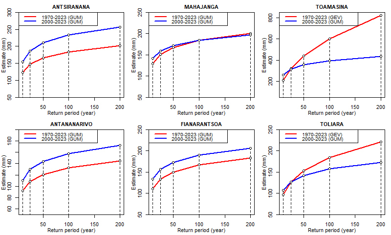Figure 4. Variability of return periods according to time series for stationary models. The return level points corresponding to return periods of 10, 25, 50, 100 and 200 years are indicated

With these models, the return periods of the maximum annual daily rainfall for each city were calculated by considering them in a 1970-2023 series and then in a 2000-2023 series, and the results are shown in Table 5.

Table 5. Return period of P24H max according to the series studied (stationary cases)

Although the results in Table 5 are consistent with the return level curves obtained by modelling with stationary GEV and/or Gumbel models (Figure 5), they present several inconsistencies with existing practical results. The most glaring is probably the fact that the same return level (for example 235.05 mm at Antsiranana) can have return periods as far apart as 732.3 years and 104.4 years with the two time series considered. The same applies to the other towns. When the return period values are fairly close (case of Toamasina), these values are abnormally low.

Figure 5 shows the example of Antananarivo, where the maximum rainfall on 22/01/2022 caused controversy over the value of the corresponding return period:

Figure 5. Case of Antananarivo for stationary models but for different time series

These results demonstrate the dependence of the return period on the size of the time series for stationary models. Moreover, with the plotting position method, the empirical probability of excess is calculated by empirical formulae in which the size of the time series appears in the denominator, as for example [34] :

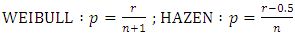(8)

being the rank of the sample values in descending order. The corresponding return period being calculated as this return period increases when the size increases.

As for the abnormally high values when we are in the presence of a GEV distribution, this can be explained by the fact that Gumbel models have an exponential growth towards infinity whereas GEV models have a power growth towards infinity. Expressed in terms of regression equations, we would therefore obtain equations of the form:

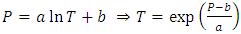(9)

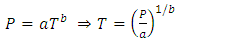(10)

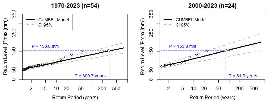
for a Gumbel distribution and a GEV distribution, respectively, and where and are regression constants to be determined and and denote the corresponding precipitation and return period, respectively.

Although the results obtained above are fairly consistent with the literature as a whole on the subject, it is worth noting a contrary result in a recently published article [27] in which, for a return period of 100 years and with the 1951-2020 (70-year) and 1991-2020 (30-year) series, it was rather the shorter time series that provided higher return level values. It should be noted that the authors of the article were themselves surprised by these results, and we believe that this is probably a special case.

The conclusion that can be drawn for stationary models is that they are intimately dependent on the length of the time series studied and give completely different or even unrealistic results for return levels and/or return periods. When the series is long and includes non-stationarity effects such as trends due to climate change, as is the case here, stationary models are no longer reliable [12,14].

4.4. Results for Non-Stationary Models

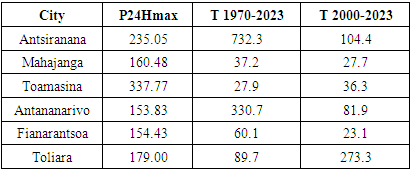
It should be remembered that in the non-stationary case, only the 1970-2023 series are analysed. Thus, by applying equations (1) and (2) for the definition of the distributions but with the parameters varying as a function of time as indicated by equations (5), (6) and (7), the best model having been chosen according to the AIC criterion (equation (8)), the results gave Table 6.

Table 6. Best non-stationary model and parameter values

As already indicated in Section 3.6, the return levels for a non-stationary model depend on the probability with which the quantile is calculated. The results are shown in Table 7.

Table 7. Return level by town for different return periods and different risk levels (non-stationary cases)

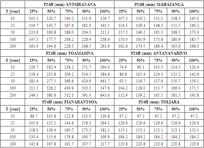
It can be seen from Table 7 that the values of the return levels for a given return period are identical for the town of Toliara because the best model for this town is a stationary GEV (Table 6).

The results in Table 7 are easier to read in graphical form (Figure 6).

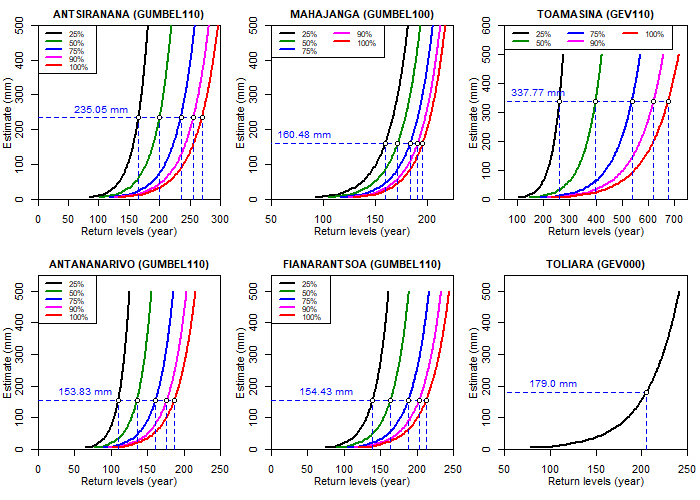Figure 6. Estimates of return periods for maximum rainfall using non-stationary models (1970-2023 series) according to risk level

The interpretation of Table 7 is a little confusing because we are used to having a single value of the return level for a return period whereas Table 7 shows that for the same value of the return period, we have different values according to the probability values (25%, 50%, 75%, 90% and 100%). These are in fact the uncertainty limits of the return periods derived from the a posteriori probabilities [35], which can also be considered as the risk level [12].

Because of the difficulty of interpreting them in the non-stationary context, several researchers have proposed abandoning the terms "return level" and "return period" and instead talking about quantiles [36] or the probability of occurrence in a given year [37]. In any case, the concept of return period merits serious revision in the non-stationary case [12].

To remain in the tradition of a single return period to be used in infrastructure design, for example, some authors propose the value of the third quartile (75%) for the final return level [12]. However, for the remainder of this work and in the second article, we have chosen to consider two levels of risk: a median level of risk (50%) and a high level of risk (90%). It will then be up to the user to choose what he feels is consistent with reality in the field.

5. Conclusions

From a set of 132 measurement points, six sites corresponding to Madagascar's provincial capitals were studied in terms of maximum annual daily rainfall for two time series: 1970-2023 (54 years) and 2000-2023 (24 years). Firstly, it was shown that there are trends in each of these series for the six towns, trends that can be attributed to climate change. Next, the break year was determined, and this break year was between 1996 and 1998, except for the city of Toliara, where the break year occurred in 1994. Using the annual maxima method (Maxima Blocks), stationary models of the distribution of extreme values were first applied to each of the two series, which showed that the best models were all Gumbel models for the 2000-2023 series and that there had been two GEV models for the 1970-2023 series, these two GEV models corresponding to the cities of Toamasina and Toliara. Calculated for return periods of 10, 25, 50, 100 and 200 years, the return levels obtained for these stationary models had given unrealistic and inconsistent values depending strongly on the size of the sample treated.

Next, non-stationary models were defined for the 1970-2023 series, the non-stationarity being translated by linear functions of time of the parameters of location and scale which led to eight possible models. The best models obtained were used to calculate the different return levels corresponding to different return periods and, similarly, the return periods corresponding to the maximum observed rainfall were determined. Some authors then indicated that the notion of return period no longer had much meaning and that it should be associated with risk levels.

However, a question that we believe to be fundamental remains unanswered: with or without stationarity, i.e. with or without taking the trend into account, what is the optimum size for the time series of extreme precipitation so that the modelling produces reliable results that are worthy of confidence? Without directly answering the question, a justification was provided by Gentilucci et al, 2023 [27], who stated that the dependence of the return value calculated with the GEV method on a longer or shorter data record is not yet sufficiently studied in the scientific literature, although it could be decisive in the choice of the length of the time series.

To avoid these problems with return levels and return periods, when sizing sensitive infrastructures or determining flood zones, the safest method is probably to carry out hydrological modelling followed by hydrodynamic modelling to determine the flows to be taken into account based on a known maximum flood event, even if it means then increasing the flows found. But this requires a great deal of effort and time.