-
Paper Information
- Next Paper
- Paper Submission
-
Journal Information
- About This Journal
- Editorial Board
- Current Issue
- Archive
- Author Guidelines
- Contact Us
Resources and Environment
p-ISSN: 2163-2618 e-ISSN: 2163-2634
2022; 12(2): 47-58
doi:10.5923/j.re.20221202.02
Received: May 23, 2022; Accepted: Jun. 24, 2022; Published: Jul. 15, 2022

Proposal of a Systematic Approach for the Identification of Favorable Sites and the Evaluation of the Average Hydroelectric Potential in Ungauged Watersheds with HEC-HMS - Case of the Ramena River (Madagascar)
 Abstract
 Reference
 Full-Text PDF
 Full-text HTML
Justin Ratsaramody
Laboratoire d'Hydraulique, Ecole Supérieure Polytechnique, Université d'Antsiranana, Madagascar
Correspondence to: Justin Ratsaramody, Laboratoire d'Hydraulique, Ecole Supérieure Polytechnique, Université d'Antsiranana, Madagascar.
| Email: |  |
Copyright © 2022 The Author(s). Published by Scientific & Academic Publishing.
This work is licensed under the Creative Commons Attribution International License (CC BY).
http://creativecommons.org/licenses/by/4.0/

The identification of favorable sites for hydroelectric development is always a costly and time-consuming operation when it is done starting with field measurements, especially in ungauged watersheds where no measurements (either of discharges or of headwater) are available. Thus, in this work, we propose a systematic approach in 5 steps applicable to any ungauged watershed. It is an approach within the reach of all since both the data (DEM, LULC, soil map, meteorological data) and the tools used are free: QGIS, SAGA for the GIS, R for the calculations and HEC-HMS for the hydrological modeling. To illustrate the method, the case of the Ramena River (Madagascar) is presented with the results obtained at each step. Because of its simplicity of access, the SCS-CN method is proposed in the illustration but it can be replaced by any other equivalent method. An important feature of the study is also the use of a fictitious average year in order to be placed in average conditions and thus reach the objective of evaluating the average hydroelectric potential of a selected site. With the final results being the guaranteed discharges and powers, the proposed approach allows a decision to be made on the development of a site, in isolated or hybrid configuration, and to foresee whether or not additional investigations in the field should be carried out.
Keywords: Favorable sites, Fictitious year, Hydrological modeling, HEC-HMS, SCS-CN, Guaranteed discharges
Cite this paper: Justin Ratsaramody, Proposal of a Systematic Approach for the Identification of Favorable Sites and the Evaluation of the Average Hydroelectric Potential in Ungauged Watersheds with HEC-HMS - Case of the Ramena River (Madagascar), Resources and Environment, Vol. 12 No. 2, 2022, pp. 47-58. doi: 10.5923/j.re.20221202.02.
Article Outline
1. Introduction
1.1. Background
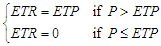
- With the ever-increasing threat to fossil fuel energy, the use of hydroelectric power can be an interesting alternative, used alone or in a hybrid configuration. Indeed, despite the Sustainable Development Goal (SDG) #7 according to which populations must have access to reliable, sustainable, modern and affordable energy services, the electrification rate in Madagascar is one of the lowest in the world: 26.9% in 2018 for the whole country and only 7.7% in rural areas (https://donnees.banquemondiale.org/indicator/EG.ELC.ACCS.ZS).Traditionally, the identification of a potential hydroelectric development site is based on the report of local residents following a visual inspection of the presence of a waterfall. Indeed, as these sites are generally far from the usual roads, their access is difficult. If the site is deemed "interesting", field trips are made for topographic and flow measurements that can take years before the data collected is statistically exploitable. Conclusions about the reliability of the site come only after a great deal of time and money has been spent, and in the batch of sites visited and measured, there are many that are rejected because they do not offer the profitability necessary for their operation. This approach is therefore empirical and unreliable.Before incurring costs for field measurements, it is advisable to know in advance which site will be of interest not only from the point of view of the head H but especially in terms of the flow rate Q, since the power that can be expected from a hydropower site is given by the relationship [1]
 | (1) |
1.2. Ramena River Location
- The Ramena River is a tributary of the Sambirano River and is located in the DIANA Region (Figure 1).
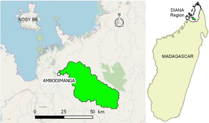 | Figure 1. Location of the Ramena River watershed with the village of Ambodimanga as outlet. On the right, location in the island of Madagascar and in the DIANA Region |
2. Materials
- The materials used are all materials that can be freely acquired on the Internet:
2.1. Data for Watershed Characterization
- To characterize the watershed, we used the following data:• Hypsometry and Hydrography: SRTM Digital Terrain Model with a spatial resolution of 30 m at watershed latitudes (https://earthexplorer.usgs.gov)• Land use and vegetation cover: Compilation of ESA Sentinel-2 2021 satellite images with a spatial resolution of 10 m [8] available at https://www.arcgis.com/ • Soil: raster file produced by the WRB (World Reference Base for Soil Resources) which is the international standard currently used by the IUSS (International Union of Soil Sciences) [9] with a spatial resolution of 250 m (HSG: Hydrologic Soil Groups) accessible on https://daac.ornl.gov/
2.2. Meteorological Data
- Weather data was obtained in time series format from https://giovanni.gsfc.nasa.gov:• Daily rainfall data TRMM_3B42_Daily v7 (Tropical Rainfall Measuring Mission) covering the period 01/01/1998 to 31/12/2019• Daily temperature data GLDAS-NOAH (Global Land Data Assimilation System) covering the period 01/01/2000 to 31/12/2019These data are averaged over an area covering a radius of 25 km, applied to the centroid of the Ramena River watershed, thus covering the entire watershed [10], [11], [12].
2.3. Computer Tools
- To carry out the calculations of reconstruction of the discharges chronicle at the outlet of the Ramena watershed, we used the following tools:• GIS processing: free software QGIS (https://www.qgis.org) and SAGA (http://www.saga-gis.org)• Programming and data processing: open source language R (https://www.r-project.org)• Hydrological modeling: HEC-HMS v. 4.6.1 (Hydrologic Engeneering Center - Hydrologic Modeling System) available at http://www.hec.usace.army.mil/software/hec-hms
3. Methods
- The approach proposed in this paper is composed of five essential steps which are, in order:• Step 1: Identification of favorable sites• Step 2: Characterization of the total river catchment• Step 3: Processing of rainfall data• Step 4: Hydrological modeling of the watershed drained by each of the sites identified in Step 1• Step 5: Exploitation of the results obtained
3.1. Step 1: Identification of Favorable Sites
- According to equation (1), the hydroelectric power obtained at a site depends on both the net head H and the discharge Q, in other words, on the topography of the land at the site and the surface drained by the watershed of which the site is the outlet. Theoretically, any site on the river could be suitable. However, for economic reasons, it is more advantageous to choose a site where the local slope is high. The higher the slope, the shorter the length of the penstock required to bring the water from the dam to the powerhouse (and therefore the lower the capital cost).Therefore, the identification of favorable sites is conducted by tracing the longitudinal profile of the river and then setting a criterion on the surface drained (> 150 km2 in our case), a criterion on the local slope (> 10% in our case) and a third criterion on the abundance of flows (presence of a major tributary upstream of the site). This longitudinal profile was drawn with QGIS from the Digital Terrain Model.
3.2. Step 2: Characterization of the Total River Watershed
- In this step, the entire river watershed must be considered, i.e., the outlet must be chosen so that the upstream portion of this outlet includes all the potential sites determined in Step 1. This step consists of classical GIS processing (with QGIS and SAGA) and the expected results are:• hypsometric characteristics and the hydrographic network• soil characteristics• Land use and land cover map (LULC)• Curve Number (CN) runoff coefficient spatial distribution mapThe objects manipulated in this step are originally rasters, but they can be easily converted to vector objects to determine their quantitative properties.The map of the spatial distribution of the CN runoff coefficient was obtained by combining the soil map and the LULC map. However, all these rasters had to be resampled beforehand in order to obtain the same spatial resolution based on the most accurate raster; in our case, this spatial resolution was 10 m (LULC raster).
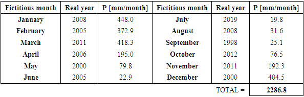
3.3. Step 3: Processing of Rainfall Data
- Even if we have a time series of rainfall data (daily rainfall from 01/01/1998 to 31/12/2019 in our case), the evaluation of the average hydroelectric potential requires that these rainfall data are also brought back to a year with average weather conditions. This average year will then be a fictitious year (say 2035) established as follows:• The fictitious month of January 2035 will be the average January from 1998 to 2019• The fictitious month of February 2035 will be the average month of February from 1998 to 2019• And so onThis gives the daily rainfall data for the fictitious year 2035.
3.4. Step 4: Hydrological Modeling
- Since the watershed is not gauged, hydrological modeling is required. For each of the identified sites, the objective of the hydrological modeling is to determine the discharge at the outlet by reconstructing the physical processes that occur in the watershed (Figure 2):
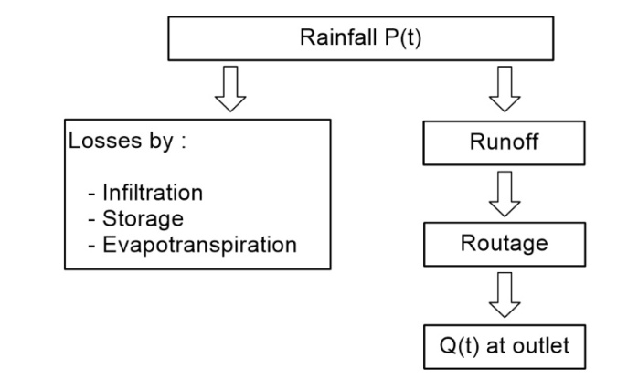 | Figure 2. Hydrologic processes for reconstructing outflow at each site |
3.4.1. Assessment of Infiltration and Storage Losses
- For this systematic approach, the recommended method for evaluating losses is the NRCS (Natural Resources Conservation Service) Curve Number (CN) method. This is a method that includes infiltration losses and storage losses but not evapotranspiration losses: it is therefore necessary to evaluate these evapotranspiration losses in another way.
3.4.2. Assessment of evapotranspiration losses
- For the evaluation of evapotranspiration losses, the method of Hamon [13] [14] can be used, which requires only easily accessible data. According to this method:
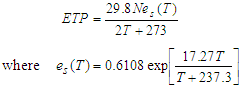 | (2) |
 : saturation vapour pressure (Pa); T: mean temperature (°C); N: number of hours of sunshine given by
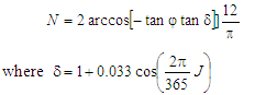 | (3) |
 | (4) |
3.4.3. Base Flow
- Base flow can be ignored if no such data is available, which is the most common case in ungauged watersheds. This would simply means that the simulated flows obtained by the hydrological modeling will actually be lower than the actual flows in the field.In our case, we had as data the specific flow
 (m3/s/km2) of the whole Ramena river catchment [15] and which corresponded to the absolute minimum daily flow (the most pessimistic value). The base flow can then be obtained by multiplying this specific flow by the area of the watershed.
3.4.4. Rainfall-Runoff Transformation Method
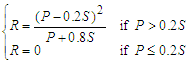
- The recommended method is the SCS-CN (Soil Conservation Service - Curve Number) runoff model associated with the SCS unit hydrograph. It is an empirical method but is among the most widely used methods in the world because of its high agreement between theoretical results and observed values. In this method, the hydrological impact of land use, vegetation cover and infiltration capacity is taken into account by a single parameter which is the CN (Curve Number). The SCS-CN model is based on the water balance equation [16]:
 | (5) |
 : initial abstraction (mm); F: cumulative infiltration (mm) which does not include
  and R is direct runoff (mm).It is furthermore assumed that there is a direct relationship between the initial abstraction and the maximum potential abstraction, S, according to [16] [17].
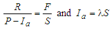 | (6) |
 | (7) |
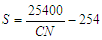 | (8) |
 | (9) |
 is the time of concentration, which is evaluated according to the Passini relationship (valid for rural watersheds larger than 4000 ha):
 | (10) |
 : Time of concentration [min].For normal (moisture) conditions, CN, denoted
  , is given by equation (8). For different antecedent conditions prior to the date of calculations, we have the following relationships [19]:
 | (11) |
 : for dry antecedent conditions and
  , for wet antecedent conditions. Generally, these conditions are for 5 days before the current day.
3.4.5. Hydrograph Routing Modeling
- The division into sub-watersheds is necessary to take into account the particularities between the different zones in the watershed of which the selected site is the outlet. This increases the accuracy of the results, particularly because of the diversity of the characteristics of these different areas: relief, flow paths, soil types, land use, soil cover, etc. After applying the loss assessment methods and the SCS-CN rainfall-runoff transformation model described above, the resulting hydrographs must be routed along the stream reaches to the outfall, i.e. the selected site.For this, the Muskingum method was used. This method is presented in the form of two equations which are the continuity equation and the storage equation at a time t [20]:
 | (12) |
 | (13) |
3.5. Step 5: Exploitation of the Results Obtained
- For each site, the results of the previous hydrological modeling lead to flow versus time records for the fictitious year. For different heads H, the expected power is then given by equation (1). These results can be processed in several ways, but the most important ones are given below.
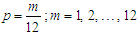
3.5.1. Empirical Probabilities
- Plotting position: by ranking the series of daily flows obtained in descending order, we can determine the empirical probabilities using, for example, the Weibull relation:
 | (14) |
 : probability of occurrence of the flow
  ; r: rank of the value
  in the series ranked in descending order; N: total number of values in the series (i.e. N = 365 for the fictive year 2035)Equation (14) thus provides the probability of occurrence of a certain flow Q0 in terms of fraction of the year. In general, the scatter plot obtained can be approximated by an empirical relationship of the form:
 | (15) |
3.5.2. Classified and Guaranteed Flows - Guaranteed Powers
- For example, for a hybrid power plant, one often needs to know for how many months one can use the power supplied by the hydroelectric plant corresponding to a given site. For this purpose, the classical way of using the classified and guaranteed flows is to replace the probability p in the adjusted expression (15) with the following values:
 | (16) |
 .Using equation (1), these flow values can be converted into power values according to the exploitable heads at each site. As for the energy produced, it can be evaluated as follows:
 | (17) |
 is the guaranteed power for m months and
  is the number of hours contained in the m months i.e.:
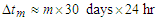 | (18) |
4. Results for Ramena River
- The method described above was applied to the Ramena River watershed (Figure 1) with the following step-by-step results.
4.1. Results of the Identification of Favorable Sites
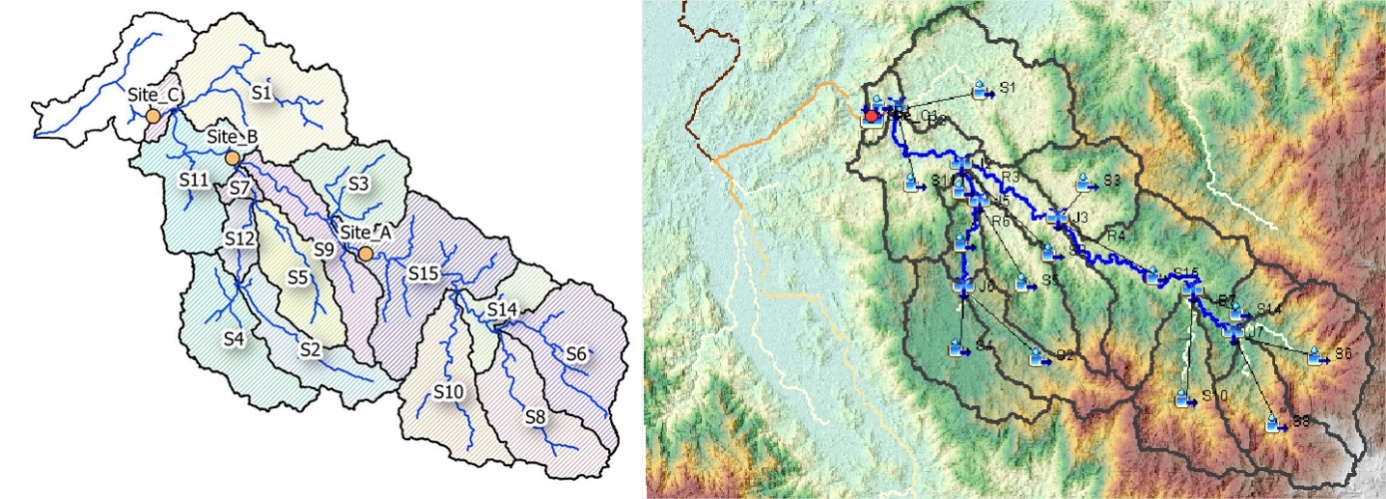
- Using the method described, three sites were identified based on the following criteria:1. Slope of the watercourse at the site > 10%.2. Watershed area drained by the site > 150 km2.3. The site is located downstream of a major tributary to benefit from additional flow inputs.By staying only on the criteria of slope, it had led to a very high number of favorable sites (148 in our case). By adding the second and third criteria above, a more reduced selection of sites could be made. We can thus see in Figure 3 that, compared to Site A, Site B benefits from the contribution of two important tributaries (Morafeno River on the right bank and Ampanasy River on the left bank). The same is true of Site C, where the inflow from the Androatra tributary is added to all the inflows from the rivers upstream.
|
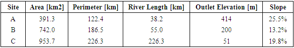
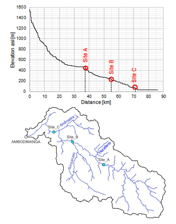 | Figure 3. Location of favorable sites. Left: Longitudinal profile of the main river. Right: Location of sites in the Ramena River watershed |
4.2. Total Watershed Characterization Results
- Hypsometric and hydrographic characteristics: Figure 4.Total length of the main Ramena river from its source to the Ambodimanga outlet: L = 86.2 km.HSG and LULC:Figure 5.Gridded CN values:Figure 6.
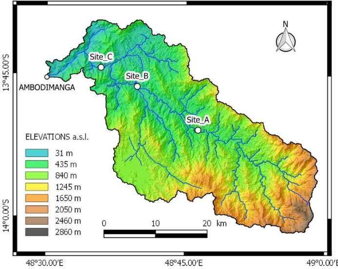 | Figure 4. Ramena River Watershed (area A = 1030 km2, perimeter P = 261 km) |
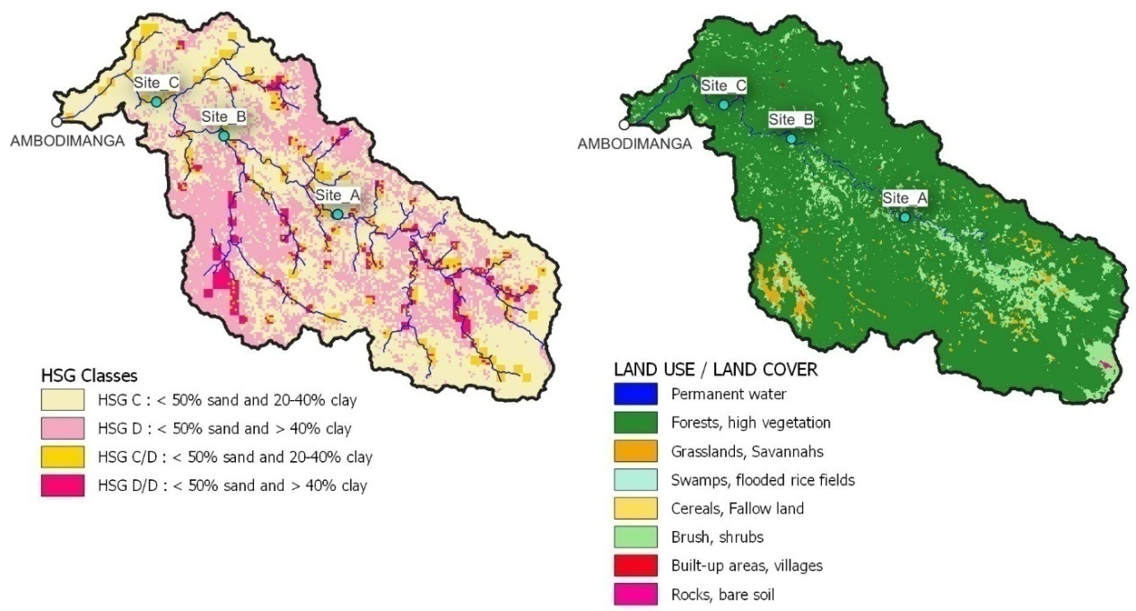 | Figure 5. Left: HSG Classes (C: moderately high runoff potentiel, D: high runoff potentiel, C/D et D/D: high runoff potentiel unless drained). Right: Land Use / Land Cover |
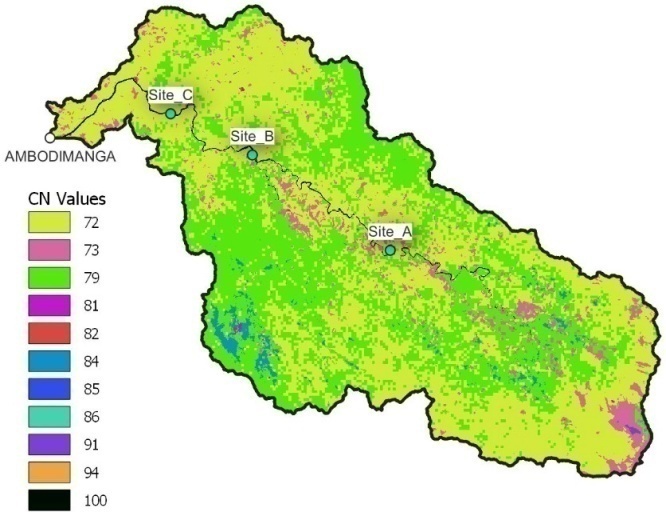 | Figure 6. Gridded CN values (random colors) |
4.3. Results of Meteorological Data Processing
- By applying the described method, the results obtained for the Ramena River are in Table 2.
|
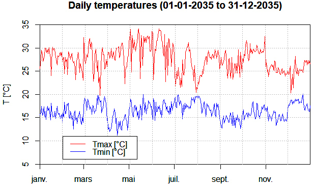 | Figure 7. Daily minimum and maximum temperatures for the fictitious mean year 2035 |
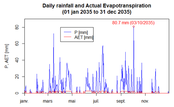 | Figure 8. Daily rainfall and real evapotranspiration for the fictitious average year 2035 |
4.4. Hydrological Modeling Results
- Division into sub-watershedsFor each of the 3 sites, the division into sub-watersheds was done automatically by the HEC-HMS software.Number of sub-watersheds:• Site A: 05• Site B: 13• Site C: 15The number of subwatersheds per site could have been reduced by merging some of them, but the more subwatersheds, the greater the accuracy.
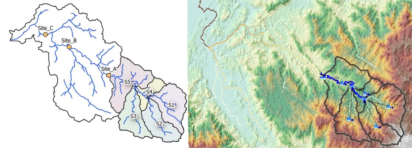 | Figure 9. Watershed of Site A divided into sub-watersheds. Left: representation in QGIS. Right: stylized representation on a terrain background in HEC-HMS |
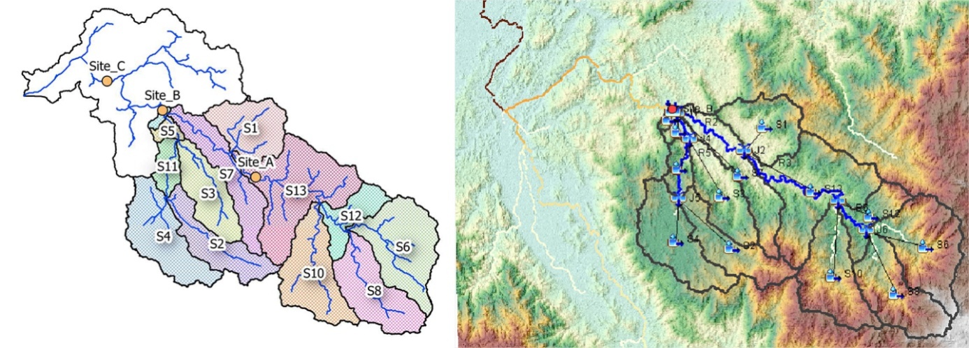 | Figure 10. Watershed of Site B divided into sub-watersheds. Left: representation in QGIS. Right: stylized representation on a terrain background in HEC-HMS |
 | Figure 11. Watershed of Site C divided into sub-watersheds. Left: representation in QGIS. Right: stylized representation on a terrain background in HEC-HMS |
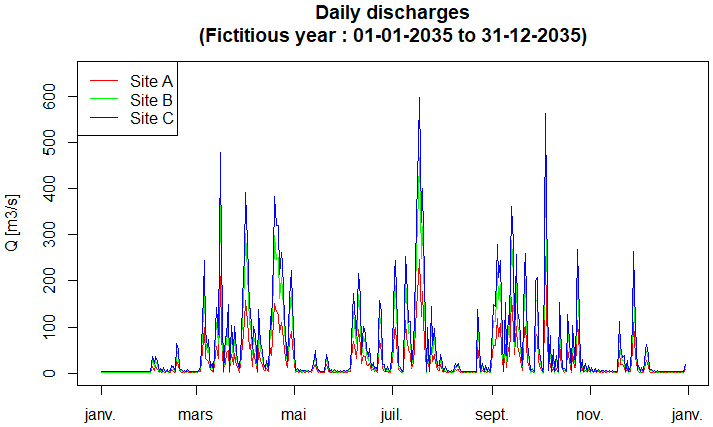 | Figure 12. Daily flows for the 3 sites in the fictitious year 2035 |
4.5. Results of the Exploitation of the Results Obtained
4.5.1. Empirical Probabilities
- By application of equation (15), the different values of the simulated flows as a function of the empirical probabilities had been fitted with an exponential curve as, for example, in Figure 13 for Site C.
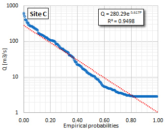 | Figure 13. Site C: simulated flows vs. empirical probabilities fitted by an exponential function |
|
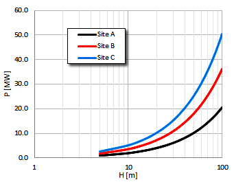 | Figure 14. Potential power P versus head H for the Ramena River |
4.5.2. Classified and Guaranteed Flows - Guaranteed Powers
- Although the curves in Figure 14 show the power that can potentially be obtained for different heads at each site, they do not provide any information on how long that power can be obtained. By applying equations (16) through (18), it is possible to determine the classified and guaranteed flows and the guaranteed powers, both as a function of time. For the illustrative case of the Ramena River, this had given Table 4.
|
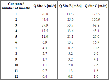
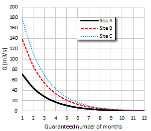 | Figure 15. Classified and guaranteed flows for the Ramena River |
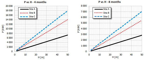 | Figure 16. Examples of guaranteed power curves as a function of head (left: 4 months; right: 8 months) for the 3 Ramena River sites |
5. Discussion of Methods and Results
5.1. On Step 1: Identification of Favorable Sites
- The use of GIS to carry out this identification had already been used by other researchers (e.g. [21], [22], [1] etc.), the fundamental difference with the present study is the addition of two other criteria, i.e. the surface drained (A > 150 km2) and the presence of a major tributary upstream of the site's outlet. Indeed, with only the criterion of slope (>10%), we had found 148 sites in the case of the Ramena River, which would have been impossible to analyze one by one. In our case, we were finally able to identify the three sites named: Site A, Site B and Site C.Very recent studies in the Philippines [26] have emphasized the importance of the spatial resolution of the DEM used, 5 m in their case, in the accuracy of the river profile. In the present study, for reasons of method reproducibility, a less spatially accurate DEM (30 m) was used, but it is much more readily available (https://earthexplorer.usgs.gov).
5.2. On Step 2: Characterization of the Total Watershed of the River
- In the hydrological model used, it was assumed that land use and land cover remained unchanged throughout the simulation (fictitious year 2035), which is not entirely true in reality [7]. This assumption had necessarily influenced the runoff results and, ultimately, the flows obtained at each site. It is possible to improve this assumption by considering month-specific LULCs from satellite image data processed by classification and averaged over the month of interest. However, this work was not necessary here since the objective was only to roughly evaluate the potential at each site before going to the field and then making the necessary measurements.
5.3. On Step 3: Processing of Rainfall Data
- The choice of using a fictitious year instead of a real year was justified by the fact that average weather conditions were to be used. It should be noted that this was based on the average months of all the observation data, which made it possible to keep the daily data corresponding to these average months. In addition, the consideration of evapotranspiration was absolutely necessary because it can be high in the Ramena River watershed [15], but this depends on the characteristics of the region under study.
5.4. On Step 4: Hydrological Modeling
- The methods we used in the hydrological modeling mainly based on the Curve Number (CN) are methods that have already been used by many studies around the world for several decades and implemented with HEC-HMS that had given acceptable results when compared to the values measured in the field. Indeed, the choice of HEC-HMS software is largely justified by its ability to model and reproduce the model and sub-models used in this study, namely a physically based conceptual model. It has also been successfully used and continues to be used for ungauged watersheds for decades by various researchers such as [2] in India, [23] in Indiana (USA), [3] in Morocco, [4] in India, [6] in Malaysia, [24] in Central Europe etc. as well as some of the researchers already mentioned above.On the question of base flow, we were fortunate to have the specific flow for the Ramena River watershed. However, even without such data, this is not a problem and can even be considered beneficial in a certain sense because it means that the flows found in the simulated hydrograph are actually lower than the actual flows, especially during the dry season.
5.5. On Step 5: Exploitation of the Results Obtained
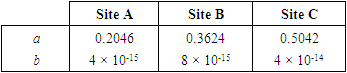
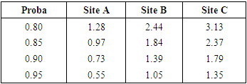
- The form of the results (classified and guaranteed flows, guaranteed powers) presented in this study is the one that assumes the use of a hybrid power plant, i.e. when another form of additional energy (thermal, photovoltaic, etc.) must be present to compensate for the insufficiencies of the purely hydroelectric energy.Some authors prefer the notion of dependable flow which is none other than the flow with a guarantee higher than 80% or 90% [1] [25] to evaluate the hydroelectric potential of a site from the FDC (Flow Duration Curve) as in Figure 13. Here, this can be done easily from equation (14) or fitting equations (15) with the parameters in Table 3 to calculate the empirical probabilities and retain only the probabilities greater than 0.8. In the case of the Ramena River, this resulted in the following Table 5:
|
6. Conclusions
- In this work, a systematic method was proposed that describes in detail how to identify sites suitable for hydroelectric development, how to evaluate the potential of each selected site and how to exploit the results obtained. In order to make it accessible to anyone and anywhere, open source data and tools were used. To illustrate this method and to describe the results to be obtained at each step, the example of the Ramena River (Madagascar), whose watershed is completely ungauged (total absence of flow measurements) was given.Despite the inaccuracies inherent to the fact that the basin is ungauged (routing parameters etc.), we believe that the method is sufficiently accurate to identify where to focus efforts and then conduct the necessary field measurements (topographic measurements to determine the head, flow measurements etc.). Once the measurements are made, these inaccuracies will be removed by calibrating the theoretical model. The method also makes it possible to foresee which type of development is possible: indeed, the flows and the guaranteed powers will allow the dimensioning of a hybrid development.Furthermore, once one or more sites are identified, the next step would be to apply weighted economic and environmental criteria to assess the actual suitability of the site [27], particularly with respect to the electrical transmission system. Furthermore, when several sites are eligible on the same river, further environmental studies are needed as recent studies [28] have shown the influence of spatial density of small hydro facilities (< 10 MW) and environmental flow on hydro potential.For the present study, the objective of the method was to help the decision-makers on the purely technical part of the water resource, but it is obvious that other criteria, such as those indicated above, can intervene in the final choice: presence or necessity of creation of access roads, length of the electric transport and distribution network, etc.