-
Paper Information
- Paper Submission
-
Journal Information
- About This Journal
- Editorial Board
- Current Issue
- Archive
- Author Guidelines
- Contact Us
Resources and Environment
p-ISSN: 2163-2618 e-ISSN: 2163-2634
2022; 12(1): 1-10
doi:10.5923/j.re.20221201.01
Received: Feb. 10, 2022; Accepted: Feb. 25, 2022; Published: Mar. 15, 2022

Estimation of the Hydrological Potential of the Ungauged Watershed of Efaho (Madagascar) from the Daily Rainfall of an Average Year
 Abstract
 Reference
 Full-Text PDF
 Full-text HTML
Justin Ratsaramody
Laboratoire d'Hydraulique, Ecole Supérieure Polytechnique, Université d'Antsiranana, Madagascar
Correspondence to: Justin Ratsaramody, Laboratoire d'Hydraulique, Ecole Supérieure Polytechnique, Université d'Antsiranana, Madagascar.
| Email: |  |
Copyright © 2022 The Author(s). Published by Scientific & Academic Publishing.
This work is licensed under the Creative Commons Attribution International License (CC BY).
http://creativecommons.org/licenses/by/4.0/

The waters of the Efaho River (Anosy Region, Madagascar) are planned to be diverted to provide water to the populations of this Androy Region who have been suffering from chronic drought for several decades. It was therefore necessary to know the value of the guaranteed flow in order to size the water transport pipes, but there are no recent measurements of flows to guarantee the hydraulic development. Thus, this study concerned the estimation of the hydrological potential of the ungauged Efaho catchment area, i.e. determining the average daily discharges of a year considered as an average year. On the daily rainfall data available from 01/01/1998 to 31/12/2019, two average daily rainfall years were considered as inputs for the hydrological model, namely the real average year 2000 and a fictitious average year, say 2053. The actual dry year 2016 was also considered. From the processing of these rainfall data, the physical processes (infiltration, evapotranspiration, runoff and then routing) had been reconstructed considering the characteristics of the catchment area. The implementation was carried out with the R language for data processing and with the HEC-HMS software for hydrological modelling. After comparison with some historical data, the results showed a fairly good agreement and the flow that could be used for hydraulic engineering was the flow corresponding to the first quartile of the fictitious average year 2053, i.e. 1.60 m3/s (guaranteed 274 days in the year).
Keywords: Ungauged catchment, Efaho, R, HEC-HMS, SCS-CN, Fictitious average year
Cite this paper: Justin Ratsaramody, Estimation of the Hydrological Potential of the Ungauged Watershed of Efaho (Madagascar) from the Daily Rainfall of an Average Year, Resources and Environment, Vol. 12 No. 1, 2022, pp. 1-10. doi: 10.5923/j.re.20221201.01.
Article Outline
1. Introduction
- The Efaho River (Anosy Region) is of paramount importance to the current government of Madagascar which has decided to divert its waters for the benefit of the populations living in the South of Madagascar, which has been suffering from chronic drought for decades, causing famine, extreme impoverishment, high infant mortality and even migration to other parts of Madagascar. These diverted waters will provide drinking water for the population as well as water for agricultural activities, livestock watering etc. Nevertheless, for the purposes of hydraulic design, it was essential to know the availability of the water resource provided by the catchment area at the point of capture. Indeed, if this resource was overestimated, the pipeline flows might not work; on the other hand, if this resource was underestimated, this would lead to water deprivation for the beneficiary populations.Figure 1 shows a general location of the Efaho catchment area. The water diverted from the Efaho River is intended to be transported to Amboasary Atsimo (Figure 1).
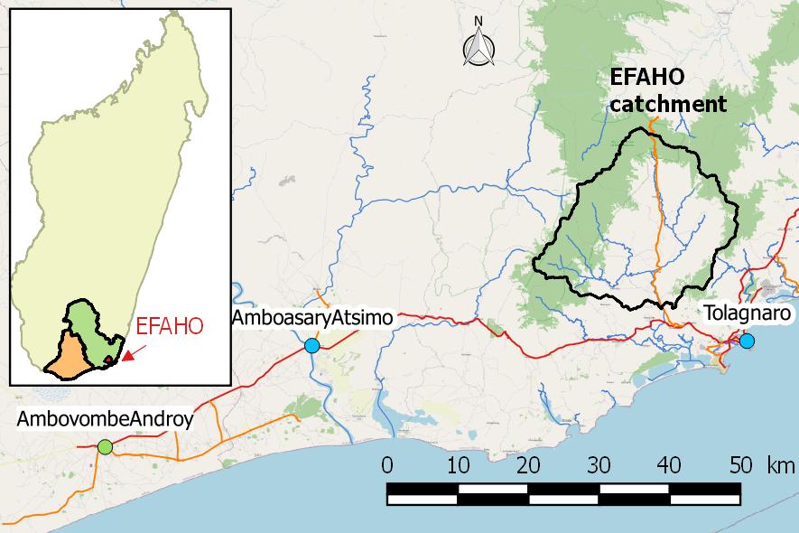 | Figure 1. General location of the Efaho catchment on an Open Street Map background. The inset shows the location of the two regions (Anosy in green and Androy in orange) concerned on the island of Madagascar |
2. Materials
2.1. Data for Catchment Characterisation
- To characterise the catchment area, the following data were used:• Hypsometry and Hydrography: SRTM Digital Terrain Model with a spatial resolution of 29 m at catchment latitudes (https://earthexplorer.usgs.gov)• Land use and land cover: Compilation of ESA Sentinel-2 2020 satellite images with 10m spatial resolution [7]• Soilology: raster file produced by the WRB (World Reference Base for Soil Resources) which is the international standard currently used by the IUSS (International Union of Soil Sciences) [8]
2.2. Weather Data
- The weather data was obtained in time series format from https://giovanni.gsfc.nasa.gov :• Daily rainfall data TRMM_3B42_Daily v7 (Tropical Rainfall Measuring Mission) covering the period 01/01/1998 to 31/12/2019• Daily temperature data GLDAS-NOAH (Global Land Data Assimilation System) covering the period 01/01/2000 to 31/12/2019These data are averaged over an area covering a radius of 25 km, applied to the centroid of the Efaho catchment and therefore cover the entire catchment ([9]; [10]; [11]).
2.3. Computer Tools
- To carry out the calculations of the reconstruction of the chronicle of the flows at the outlet of the Efaho catchment, the following tools were used:• GIS processing: free software QGIS (https://www.qgis.org) and SAGA (http://www.saga-gis.org)• Programming and data processing: open source language R (https://www.r-project.org )• Hydrological modelling: free software HEC-HMS v. 4.6.1 (Hydrologic Engeneering Center - Hydrologic Modeling System) available at http://www.hec.usace.army.mil/software/hec-hms
3. Methods
3.1. Catchment Characterisation
- The geometric, hypsometric and hydrographic characteristics of the catchment area were obtained by processing the DTM. Land use and land cover (LULC) were obtained from the above data using the visible spectral bands (blue, green, red), the near infrared band and two shortwave infrared bands [7].
3.2. Rainfall Data Processing: Real or Fictitious Average Year
- In order to determine the average daily flow record, the rainfall data used should be that of a year with "average" weather conditions, especially with regard to rainfall. To select this year of average conditions, two methods can be used:a) Either the real average year is considered, which corresponds to the average precipitation year over the 22 years of observations (1998 to 2019)., which corresponds to the average rainfall year over the 22 years of observations (1998 to 2019)b) Or a fictitious average year is created which is determined in the following way:• for each month (January, February etc.) and for the 22 years (1998 to 2019), the monthly average daily rainfall was determined• the month of the year corresponding to this monthly average thus constitutes the month of the fictitious year which is then composed month by month in this wayThe average year thus determined, whether real or fictitious, will then be the daily rainfall series that will constitute the input data for the hydrological modelling. By proceeding in this way, exaggerations are avoided that could have been caused by the great variability of rainfall from one year to the next. Nevertheless, the dry year is also considered, i.e. the year with the lowest annual value among the years of observation.
3.3. Assessment of Evapotranspiration
- Rainfall loss rates through evapotranspiration can be high in the dry season [1], so it was essential to take this into account.For the calculation of potential evapotranspiration (PET), the formula of Hamon ([12], [13]) was adopted:
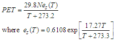 | (1) |
 : potential evapotranspiration (mm);
  : saturation vapour pressure (Pa);
  : mean temperature (°C);
  : number of hours of sunshine given by
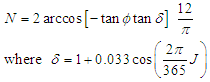 | (2) |
 | (3) |
3.4. Modelling of Rainfall-Runoff Transformation Processes
3.4.1. SCS-CN Runoff Model
- In this work, the SCS-CN (Soil Conservation Service - Curve Number) runoff model was adopted which, although empirical in nature, is one of the most widely used methods in the world due to its high agreement between theoretical results and observed values. Another reason for its popularity is that the model depends on a single parameter, CN, which reflects the hydrological impacts of land use, land cover and infiltration capacity. The SCS-CN model is based on the water balance equation [14]:
 | (4) |
 : initial abstraction (mm); F: cumulative infiltration (mm) which does not include
  and R is direct runoff (mm).With the additional assumption of a direct relationship between the initial abstraction and the maximum abstraction potential, S, it leads ([14]; [15])
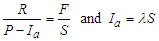 | (5) |
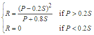 | (6) |
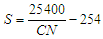 | (7) |
 | (8) |
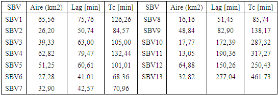
 is the time of concentration.The time of concentration
  was evaluated (for each of the sub-catchments) according to Passini's relationship (valid for rural watersheds with a surface area of over 4000 ha):
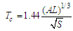 | (9) |
 : Time of concentration [min].For normal (moisture) conditions, the CN, denoted CN(II), is given by equation (7). For different past conditions prior to the date of calculation, the following relationships exist [16]:
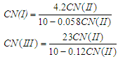 | (10) |
3.4.2. Baseflow Modelling
- Researchers have already addressed the issue of determining baseflow, e.g. [19] for Ontario (Canada), unfortunately all proposed methods were based on the existence of regional data with gauged catchments. Thus, in the absence of measurements, this baseflow was evaluated monthly as being the flow corresponding to 15% of the flows calculated without base flows, an arbitrary but realistic value in view of the impermeable behaviour of the basin [1] in which the water tables play a minor role.
3.5. Hydrograph Routing Modelling
- In general, the routing of hydrographs of flows at the outlet of the various sub-catchments is based on the Saint-Venant equations [20]
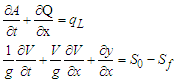 | (11) |
 = energy line slope;
  = bed slope; V = velocity; y = hydraulic depth; x = distance along the flow path; t = time; g = acceleration due to gravity;
  : lateral flow per unit length.In the present study, the model adopted was the Muskingum model which is obtained by combining the continuity equation and the diffusive representation of the Saint-Venant momentum equation, i.e. by neglecting the convective acceleration (V/g)(∂V/∂x) and the local acceleration (1/g)(∂V/∂t) in the dynamic equation i.e.:
 | (12) |
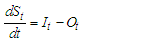 | (13) |
 | (14) |
 : inflow to the reach (m3/s);
  : outflow from the reach (m3/s);
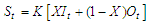
  : storage in the reach (m3); K is the storage constant (sec) and X is the weighting factor (-) between the inflow and the outflow.For routing, both equations (13) and (14) have to be numerically integrated. And at each time step and at each computational space step, the K and X parameters of the Muskingum model are recalculated based on the properties of the routing channel and the flow depth. This is necessary to ensure the stability and convergence conditions of the numerical integration (CFL condition).
4. Results
4.1. Catchment Characteristics
- The characteristics of the Efaho River catchment are shown in Figures 2, 3 and 4.
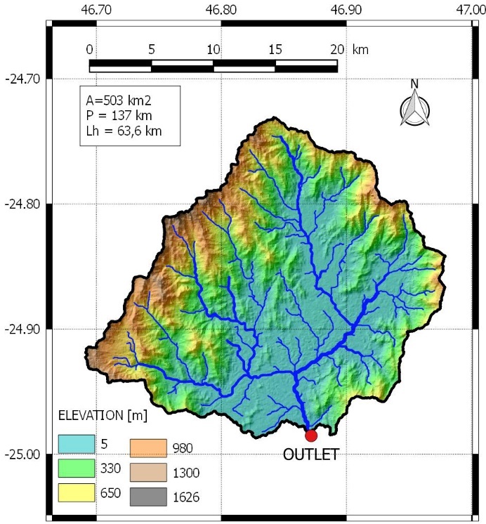 | Figure 2. Hypsometry and Hydrography of the Efaho catchment. Lh=63.6 km is the hydraulic length of the main river |
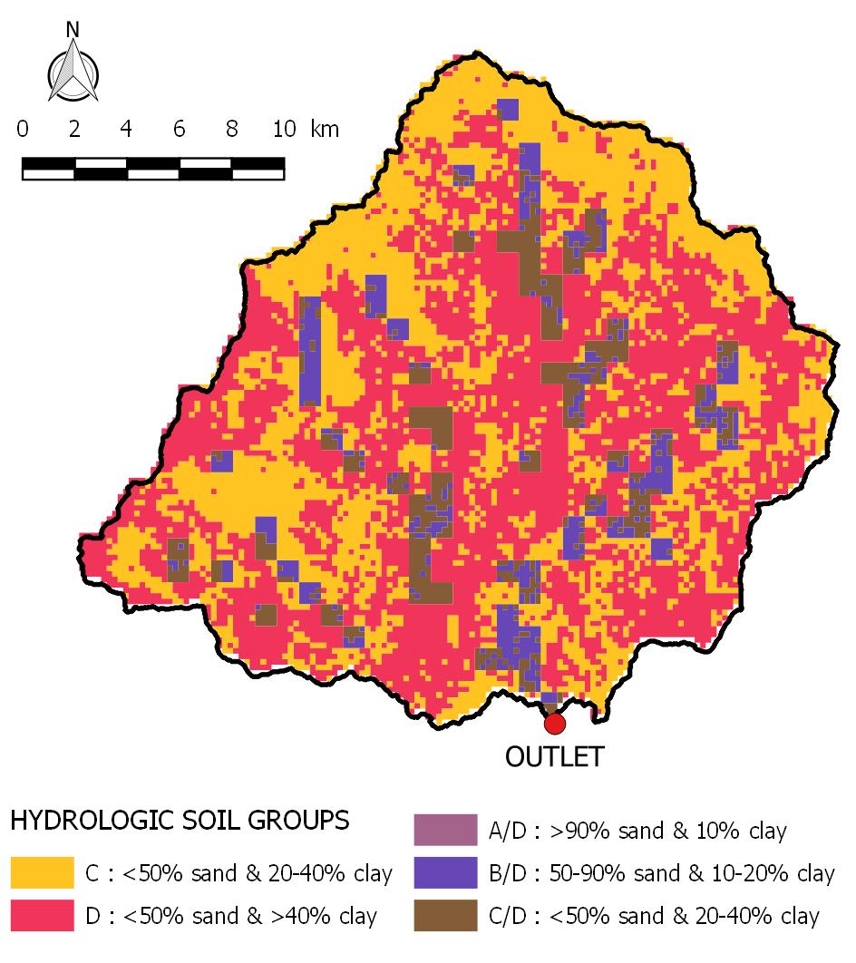 | Figure 3. Hydrological soil classes (HSG) of the EFAHO catchment: very high impermeability (dominance of Class C and Class D) |
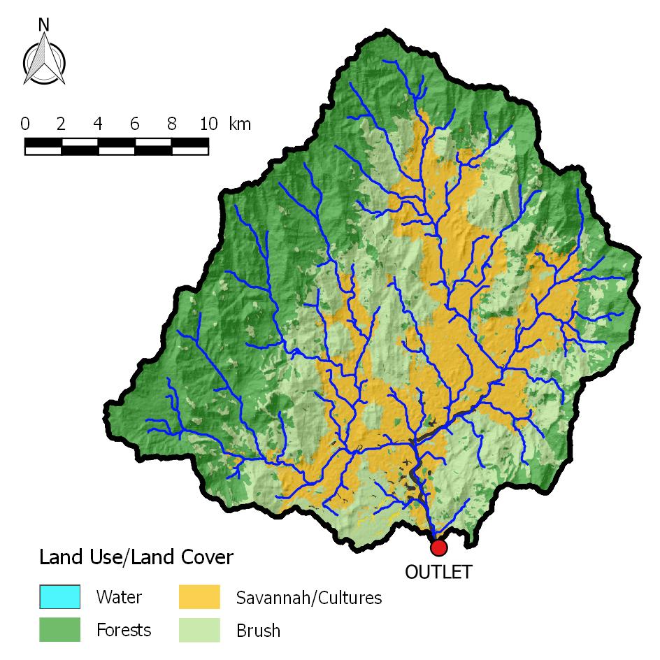 | Figure 4. Land use and land cover in the Efaho catchment |
|
4.2. Results of Meteorological Data Processing
4.2.1. Distribution of Interannual Daily Rainfall
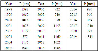
- This distribution is shown in Table 2 which shows that the average year was 2000 (2013 mm annual rainfall) while the driest year was 2016 (with an annual rainfall of 468 mm).
|
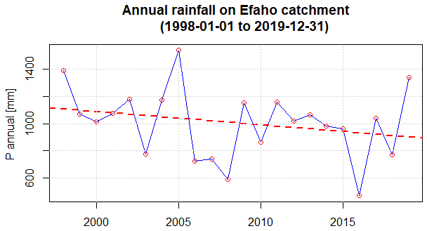 | Figure 5. Temporal variation of annual rainfall in the Efaho catchment. Red dashed line: regression line indicating the overall trend |
4.2.2. Actual Average Year and Fictitious Average Year
- Using the procedure described in § 3.2, these are the actual average year 2000 and the fictitious average year 2053 (a non-leap year date assigned quite randomly). These two time series are shown in Figure 6 and 7, respectively.
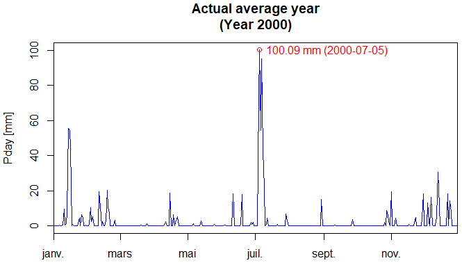 | Figure 6. Actual average year (year 2000). Annual total = 1013.1 mm; maximum value: 100.09 mm occurred on 05 July 2000 |
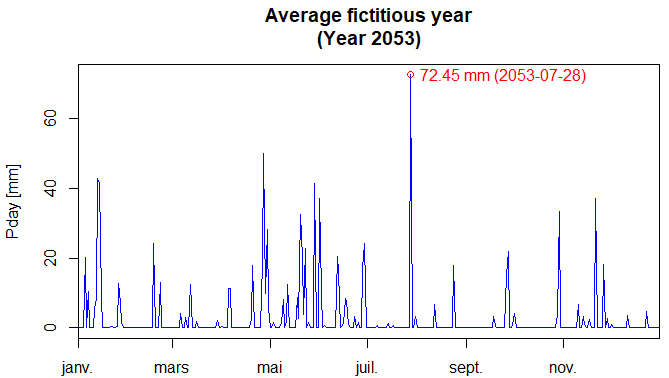 | Figure 7. Fictitious average year. Annual total = 971.5 mm; maximum value: 72.5 mm on 28 July |
4.2.3. Results of Evapotranspiration Calculations
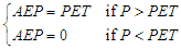
- By applying the relationships (1) to (3) with the data of the fictitious average year, the values of actual evapotranspiration (AEP) shown in Figure 8 with the daily rainfall distribution were obtained:
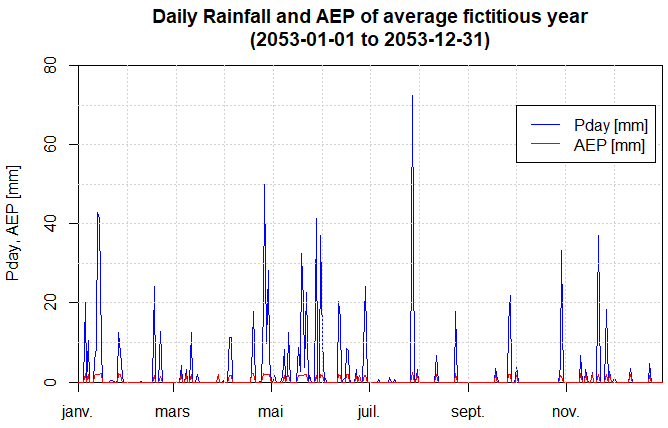 | Figure 8. Distribution of daily rainfall and AEP for the fictitious average year |
4.3. Hydrological Modelling Results
4.3.1. Division into Sub-Catchments
- In order to carry out the hydrological modelling, the Efaho catchment was divided into 13 sub-catchments (SBV) shown in Figure 9:
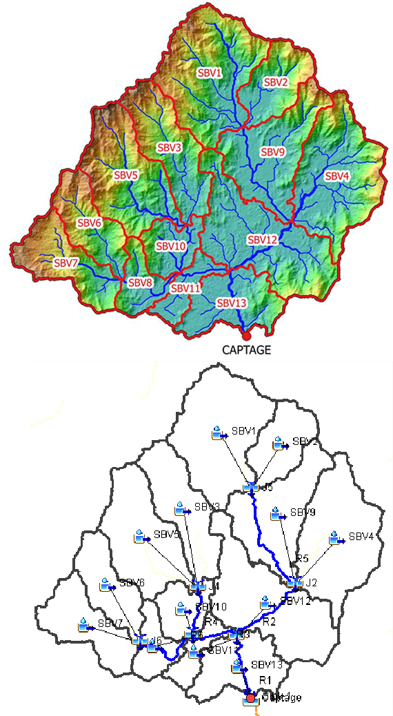 | Figure 9. Sub-catchments of the hydrological modelling. Top: representation in real space. Bottom: schematic representation in HEC-HMS |
|
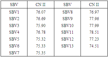
4.3.2. CN values for Sub-Catchments
- The normal CN values (CN(II)) for each of the sub-catchments are given in Table 4.
|
4.3.3. Final Results
- For the three years studied, Figures 10 to 12 show the variation of the average daily flows at the catchment site (outlet of the total catchment) considering the base flow (15% of the calculated flow):
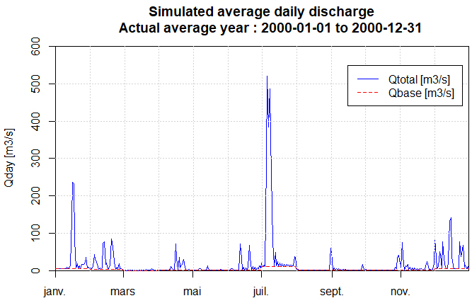 | Figure 10. Average daily flows for the actual average year (year 2000) |
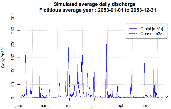 | Figure 11. Average daily flows for the fictitious average year (year 2053) |
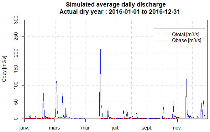 | Figure 12. Average daily flows for the actual dry year (year 2016) |
5. Discussions
5.1. Concerning the Data and Tools Used
- The data used in this work (physical characterisations, meteorological data) are data commonly used by the scientific community and their spatial resolution is sufficiently high, 29 m for the DTM and 10 m for the LULC, to consider them as very representative of the physical reality of the watershed.As regards the computer tools used (R, HEC-HMS), these are also fairly widely used tools, even if other tools could also have been used for this study. In addition to the fact that it is free of charge, the choice of HEC-HMS seemed to us to be largely justified by its capacity to model and reproduce the model and the sub-models used in this study, namely a conceptual model with a physical basis. It has also been successfully used and continues to be used for ungauged catchments for decades by different researchers such as [22] in India, [23] in Indiana (USA), [24] in Morocco, [25] in India, [26] in Malaysia, [27] in Central Europa etc.
5.2. Concerning the Processing of Rainfall Data
- Considering mainly the three years 2000, 2016 and 2053 allows for long-term operation under either "average" or "dry" conditions, the latter being critical from a safety perspective. Indeed, in the future, even if weather conditions change from one year to the next, it is unlikely that these changes will significantly affect the conditions of an average year, especially with the way the fictitious year 2053 was constructed.
5.3. Concerning the Method of Calculating PET and AET
- In the present study, the Hamon method was used ([11], [13]) mainly because of the availability of data that this method requires. The most recommended method is the so-called FAO56-PM method derived from the Penman-Monteith equation and standardised by FAO ([28], [29]). Studies by [30], on 7 years of daily data concluded that the standard error of the Hamon method compared to FAO56-PM is 0.25 mm/month, which is quite negligible.
5.4. On Hydrological Modelling
- The results of the method are dependent on the regional parameter λ as it conditions the initial abstraction and thus the storage capacity of the catchment (equation (5)). Although other researchers have found that it can be as λ = 0.05 [31], in the absence of field measurements to assess this, the value used in this study, λ = 0.2, was justified as we are in average conditions. Indeed, a low value of λ means a low storage capacity before the runoff, so there is a risk of having overestimated flows at the outlet, which can be misleading and therefore unsafe in relation to the objectives of this study.Regarding routing, the parameters K and X were also evaluated at average values (K=0.5 and X=0.25) knowing that K has a value reasonably close to the travel time of a wave on the reach (Song et al., 2011) while X a measure of the degree of storage in the river and varies from 0 (maximum storage) to 0.5 (no storage but pure transmission). It must be recognised that field measurements of river morphology would have allowed the values of K and X to be set much more precisely.
5.5. On the Final Results
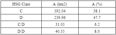
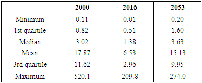
- Interpretation of the shape of the daily flow hydrographsFigures 10, 11 and 12 are very different from each other, but all three show a highly dissected appearance which is characteristic of a low base flow and individualised floods. This is due to the fact that the flow is not regulated by groundwater because the basin is practically impermeable as shown in the hydrological soil class map (Figure 3).Characteristic statistical valuesThe main characteristic values of the temporal flow distributions are summarised in the table below:
|
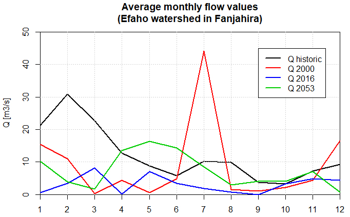 | Figure 13. Comparison of monthly average flows with historical data |
|
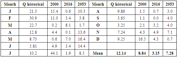
5.6. Choosing an Average Year for Hydraulic Operation
- In terms of hydraulic use of the flows generated at the outlet, the fictitious average year (2053) can be a good representation of the catchment potential. In this case, the flow to be based on would be the flow corresponding to the 1st quartile, i.e. 1.60 m3/s (guaranteed for 274 days). Indeed, the actual dry year 2016 is too pessimistic while the actual average year 2000 is only the average over the period considered (1998 to 2019) but this will certainly no longer be the case in the years to come.
6. Conclusions
- The present study was concerned with the assessment of the hydrological resources of the Efaho catchment. Free data were used for hypsometry, hydrography, land use, land cover, pedology and meteorological data. The assessment was based on the reconstruction of the physical processes (evapotranspiration, infiltration, runoff, routing) that give rise to the hydrograph of daily flows at the outlet.For this assessment, the method for transforming rainfall into runoff was the SCS-CN method and the SCS unit hydrograph. For the routing method, the so-called Muskingum method was chosen. The implementation of the defined model was carried out with the HEC-HMS software and the computer programs were coded with the R language.Throughout this study, flows for a dry year (2016) and two average years (real average year 2000 and fictitious average year 2053) were calculated. Likewise, the parameters used were average parameters, particularly with regard to the Muskingum K and X parameters.Finally, a comparison with historical data was made for a fraction of the catchment area. This comparison showed that the same conclusions were reached from a qualitative point of view, but quite different from a quantitative point of view due to different assumptions and methods.We recommended considering the average fictitious year 2053 for a hydraulic exploitation of the generated flows. However, in the absence of field measurements, the results of the present study are theoretical and the rainfall-discharge transformation models are uncalibrated models. An undeniable improvement of these models would be to carry out flow measurements at the outlet, which would make it possible to calibrate the real value of the parameters instead of simply considering average values.