-
Paper Information
- Next Paper
- Paper Submission
-
Journal Information
- About This Journal
- Editorial Board
- Current Issue
- Archive
- Author Guidelines
- Contact Us
Resources and Environment
p-ISSN: 2163-2618 e-ISSN: 2163-2634
2017; 7(6): 145-159
doi:10.5923/j.re.20170706.01

Modelling the Effect of Land Use and Land Cover Variations on the Surface Temperature Values of Nairobi City, Kenya
 Abstract
 Reference
 Full-Text PDF
 Full-text HTML
Maurice Onyango Oyugi1, Faith N. Karanja2, Victor A. O. Odenyo3
1School of the Built Environment, Department of Architecture and Building Science, University of Nairobi, Nairobi, Kenya
2School of Engineering, Department of Geospatial and Space Technology, University of Nairobi, Nairobi, Kenya
3School of Environmental Studies, Department of Environmental Monitoring, Planning and Management, University of Eldoret, Eldoret, Kenya
Correspondence to: Maurice Onyango Oyugi, School of the Built Environment, Department of Architecture and Building Science, University of Nairobi, Nairobi, Kenya.
| Email: |  |
Copyright © 2017 Scientific & Academic Publishing. All Rights Reserved.
This work is licensed under the Creative Commons Attribution International License (CC BY).
http://creativecommons.org/licenses/by/4.0/

Urbanization replaces natural vegetation with impervious surfaces such as roads and buildings. Since impervious surfaces have higher thermal energy absorption and retention capacities, they store thermal energy during the day and slowly released it at night. The energy exchange in conjunction with anthropogenic heat contributes to the development of urban heat islands. To establish the relationship existing between urban surface temperature values, land uses and land covers, information on the same provided by Landsat TM imageries of the years 1988 and 1995 as well as Landsat ETM+ imageries of the years 2000, 2005, 2010 and 2015 consisting of Band 2 (Green: 0.52μm –0.60 μm), Band 3 (Red: 0.63μm - 0.69μm), Band 4 (the NIR: 0.76μm – 0.90μm) and Band 6 (10.4 – 12.5μm) were used. The objectives of this study were to establish the distribution of land uses and land covers within the city between the years 1988 to 2015,toestablish the spatial variations in surface temperature values in the city between the years 1988 to 2015 and to determine the relationship existing between the land uses and land covers of the city and the surface temperature values. To accomplish the objectives, spatio-temporal models of land uses and land covers as well as surface temperature variations within the city were evolved to aid in the postulation of a quantitative model explaining how land uses and land covers determine the surface temperature distribution in the city. This was undertaken in furtherance to theoretical postulations on the effect of urbanisation indicators notably the land use and land cover alterations on global warming and climate change.
Keywords: Surface Temperature, Urban Heat Islands, Land Use, Land Cover, Geospatial Systems
Cite this paper: Maurice Onyango Oyugi, Faith N. Karanja, Victor A. O. Odenyo, Modelling the Effect of Land Use and Land Cover Variations on the Surface Temperature Values of Nairobi City, Kenya, Resources and Environment, Vol. 7 No. 6, 2017, pp. 145-159. doi: 10.5923/j.re.20170706.01.
Article Outline
1. Introduction
- Higher urbanization rates present a major challenge to urban sustainability especially to the developing countries which are characterised by low technical and financial capacities for urban environmental management. In the recent decades, realisation that global warming and climate change is accentuated by increased urbanisation and greenhouse gas emissions has heightened studies on the links between urbanisation indicators such as development densities, land uses, land covers and the urban environmental quality parameters such as the urban heat islands, air quality, climate change and global warming. Some of these studies posit that a proportion of the 0.5°C global warming seen over the last century is attributed to increased urbanization (Kukla et al., 1986; Changnon, 1992; Wood, 1988; Jones et al., 1990; Wigley and Jones, 1988; Nasrallah and Balling, 1993). The urban land uses and land covers notably the buildings and the green belts attenuate wind flow within the urban canopy layer which in turn affects the distribution of the urban thermal values. The above explains the occurrence of higher surface temperature values in the cities relative to their hinterlands. Scholars therefore agree that there is a significant relationship existing between urban land uses, land covers and the surface temperature values. The fundamental question is therefore to what extent are land use and land cover parameters of urban built-up, open and transitional areas as well as vegetation cover determines the spatial distribution of the surface temperature values within the city (Chan et al., 2003; Givoni, 1998; Soulhac et al., 2001; Britter and Hanna, 2003; Golany, 1996; Karatasou et al., 2006).
2. The Aim and Objectives of the Study
- The aim of this study was to establish the relationship existing between the land use, land cover and the surface temperature values of Nairobi city as derived from geospatial measurements. This was undertaken in furtherance to the postulations on the effects of urbanisation on global warming and climate change. Accordingly, the objectives of the study were: -i. To establish the distribution of land uses and land covers within the city between the years 1988 to 2015, ii. To establish the spatial variations in surface temperature values in the city between the years 1988 to 2015, iii. To determine the relationship existing between the land uses and land covers of the city and the surface temperature values.
3. Methods and Materials
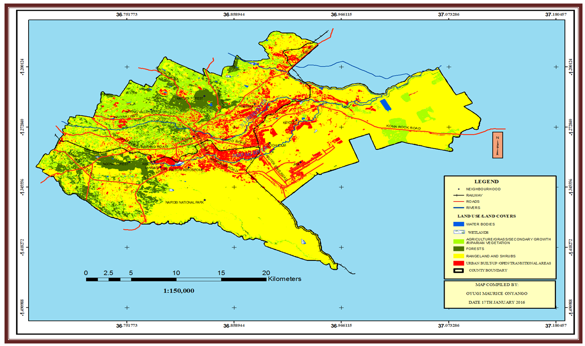
- This study adopted both descriptive and quantitative research designs. While descriptive designs are concerned with explaining who, what, when and how a phenomenon occurs over space, quantitative designs explains how various factors affecting an occurrence of a phenomenon are related (Babbie, 2002; Cooper et al., 2003). In this study, the entire land surface constituting the jurisdictions of the Nairobi City County Government which is bounded within the longitudes 36° 40’ and 37° 10’E and between latitudes 1°09’ and 1° 28’S covering an area of 716 km2 constituted the target population. Sampling was inappropriate for the imageries used in the study had full spatial coverage of the city.
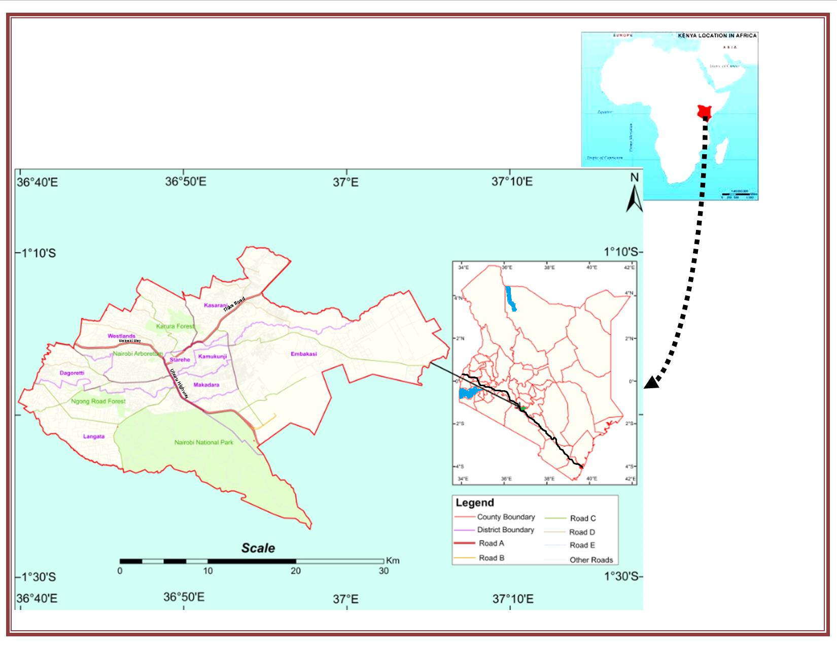 | Figure 1. The Study Area |
|
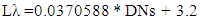 | (1) |
 | (2) |
 The fourth step involved the calculation of the Normalized Differential Vegetative Indexes (NDVIs) using the below stated function.
 | (3) |
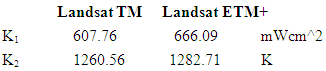
 | (4) |
 | (5) |
4. Findings and Discussions
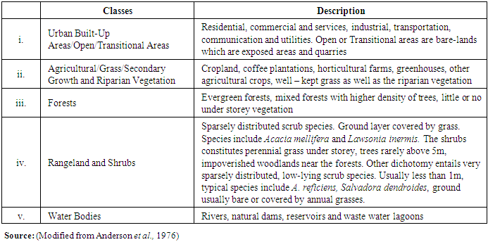
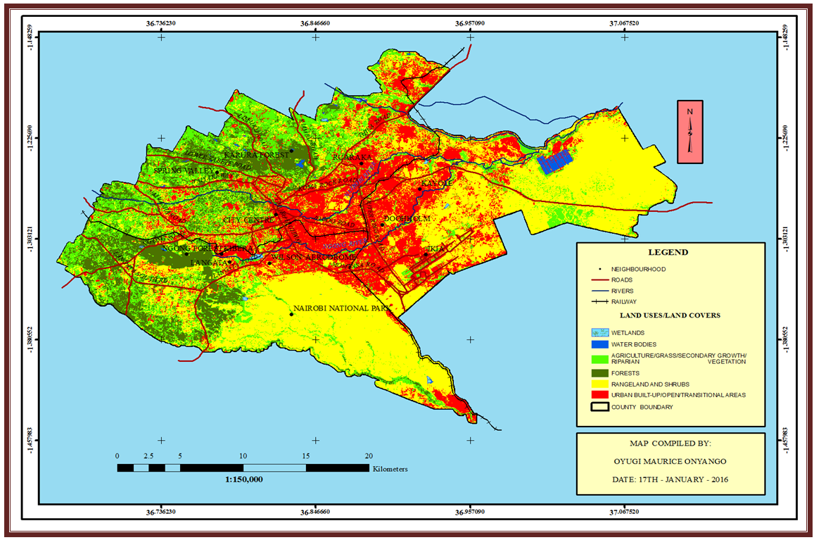
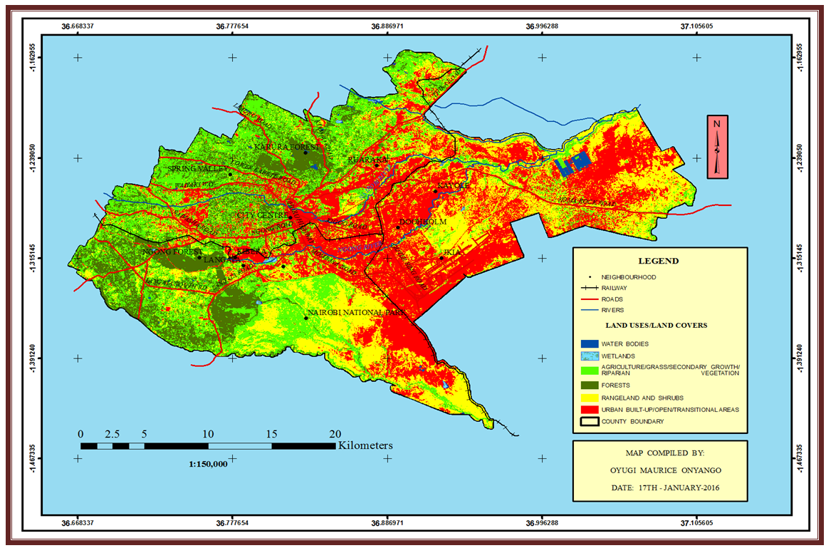
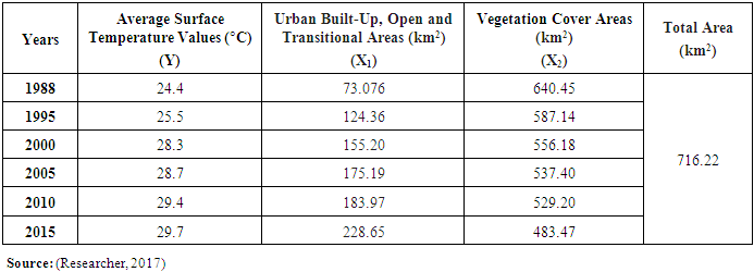
- Land Uses and Land Covers of Nairobi City for the Period between 1988 and 2015The classified land use and land cover maps of Nairobi for the years 1988, 1995, 2000 2005, 2010 and 2015 are shown in Figures 2, 3, 4, 5, 6 and 7 respectively. While quantification of land uses and land covers is summarized in Table 2, trends of the same are presented in Figure 8. This study reveals that the area of the city under built-up, open and transitional land cover have increased from 73.08 km2 in the year 1988 to 228.65 km2 in the year 2015. While agricultural, grass, secondary growth and riparian vegetation which occupied 126.82 km2 of the city in the year 1988 have marginally increased to 189.73 km2 in the year 2015; forest cover have shown mixed gains and loss. In the year 1988, the area of the city under the forest cover was 59.63 km2. This increased to 122.41 km2 in the year 1995 and thereafter declined by approximately 52% reaching 63.63 km2 in the year 2000. The decline is attributed to the indiscriminate extraction of forest resources and clearance of the same for urban developments which characterised the periods between the years 1995 to 2002. This situation was reversed in the year 2003 when the new government re-emphasised and re-energised strategies geared towards increasing the forest cover in the country. Such strategies included the degazettement and clearance of illegal structures within the forest reserves. This has since made the area of the city under forest cover to gradually increase from 63.63 km2 in the year 2000 to 93.44 km2 in the year 2015. The area of the city under rangeland and shrub vegetation cover have steadily declined from the year 1988 when it covered 453.99 km2 of the city to 200.30 km2 in the year 2015.
 | Figure 2. Land Use and Land Cover Map of Nairobi for the Year 1988 |
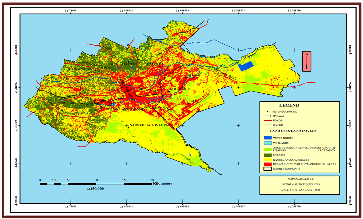 | Figure 3. Land Use and Land Cover Map of Nairobi for the Year 1995 |
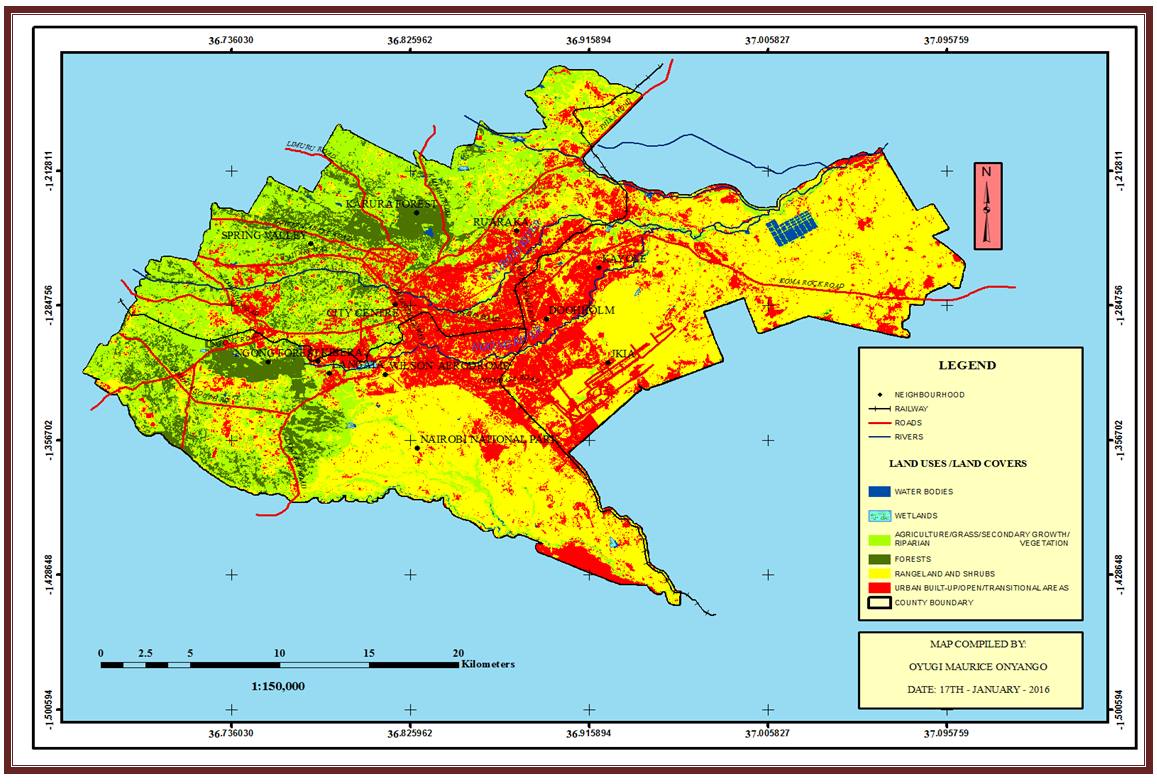 | Figure 4. Land Use and Land Cover Map of Nairobi for the Year 2000 |
 | Figure 5. Land Use and Land Cover Map of Nairobi for the Year 2005 |
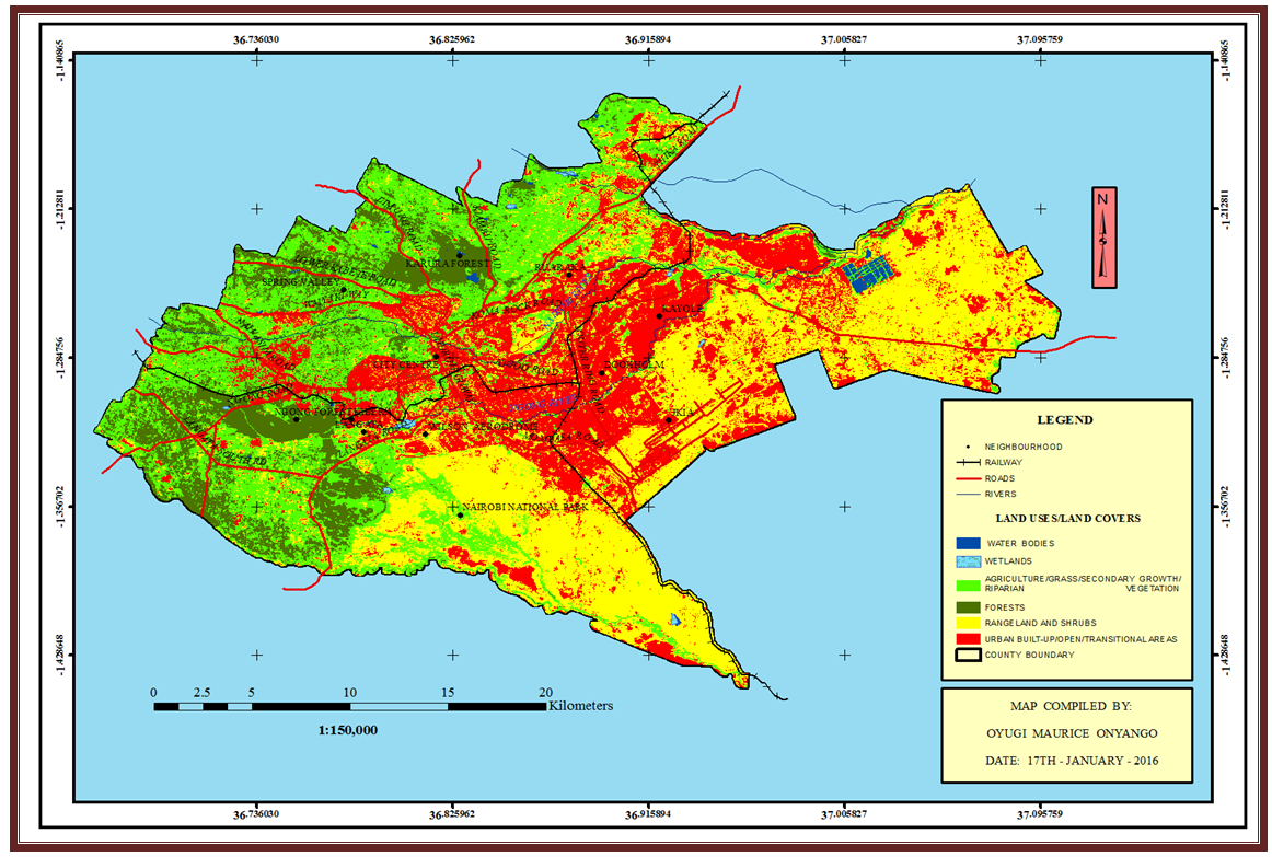 | Figure 6. Land Use and Land Cover Map of Nairobi for the Year 2010 |
 | Figure 7. Land Use and Land Cover Map of Nairobi for the Year 2015 |
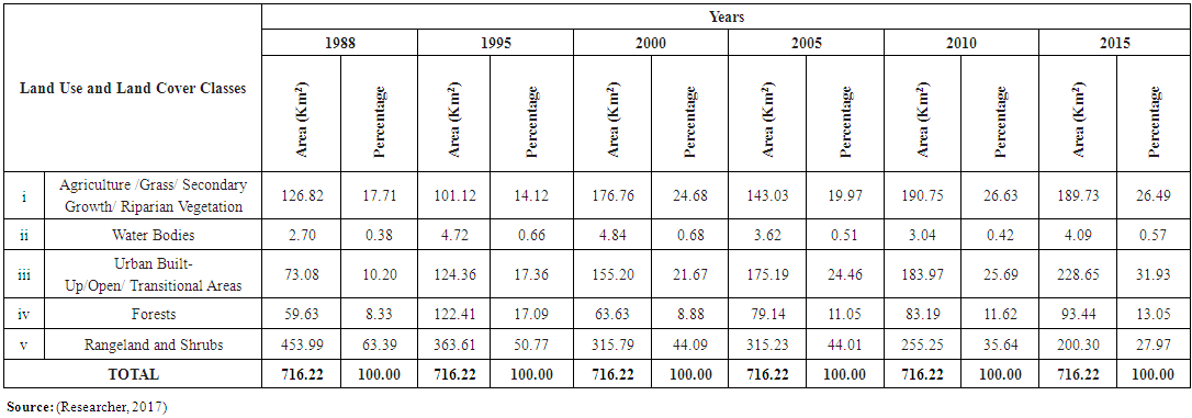 | Table 2. Land Use and Land Cover Types in Nairobi City between the Years 1988 to 2015 |
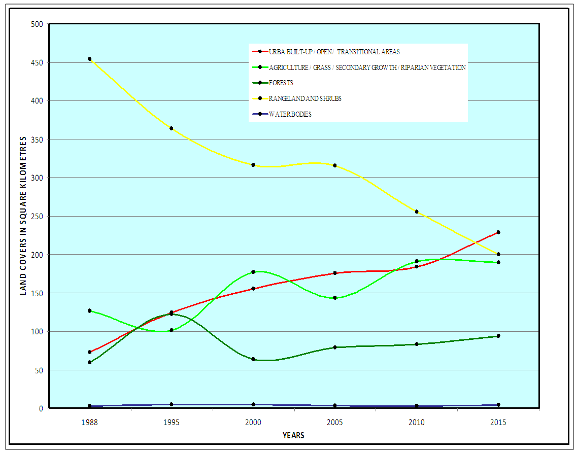 | Figure 8. Land Use and Land Cover Change Trends in Nairobi City between the Years 1988 to 2015 [Source: (Researcher, 2017)] |
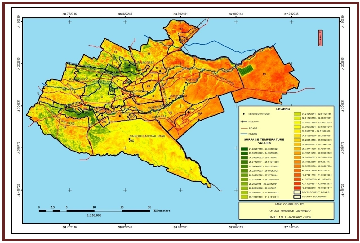
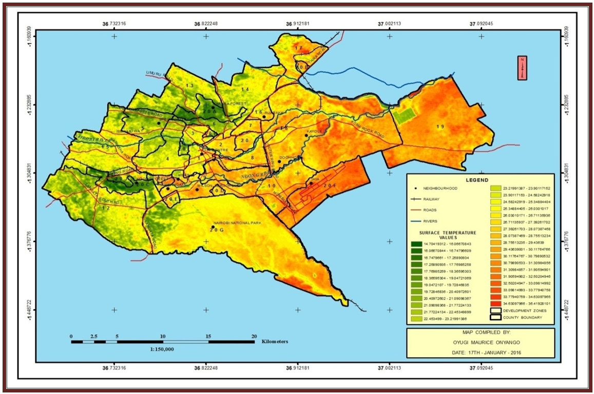
 | Figure 9. The Spatial Distribution of the Surface Temperature Values of Nairobi City in the Year 1988 |
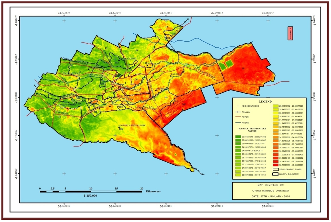
 | Figure 10. The Spatial Distribution of the Surface Temperature Values of Nairobi City in the Year 1995 |
 | Figure 11. The Spatial Distribution of the Surface Temperature Values of Nairobi City in the Year 2000 |
 | Figure 12. The Spatial Distribution of the Surface Temperature Values of Nairobi City in the Year 2005 |
 | Figure 13. The Spatial Distribution of the Surface Temperature Values of Nairobi City in the Year 2010 |
 | Figure 14. The Distribution of the Surface Temperature Values within Nairobi City in the Year 2015 |
|
 | (6) |
5. Conclusions
- This study has established that the built-up, open and transitional developments as well as vegetation cover determines the spatial distribution of surface temperature values in the city with varying levels of significance. Of the two variables considered by the study, the built-up, open and transitional development is the most significant variable influencing the spatial distribution of the surface temperature values in the city. However, if the significance of the error term in the model explaining the relationship existing between surface temperature values, the built-up, open and transitional developments and the vegetation cover has to be minimised then alongside with the stated variables, inclusion of other parameters such as topography, pedology, rainfall pattern and amount, slope, aspects and wind velocity among others should be considered in aiding the building of a comprehensive model explaining the spatial distribution of the surface temperature values in the city. This study confirms the theoretical postulations that the relationship existing between the surface temperature values, land uses and land covers of a city is hinged on intervening, indirect and direct variables such as the urban population distribution, pedology, topography, wind velocity, slope, aspects, climate (rainfall pattern and amount) of the region where the city is located, vegetation, development densities, land uses, street and building configurations (Sundarakumar et al., 2011; Mahmood et al., 2010; Tan et al., 2010; Gottdiener and Budd, 2005).
ACKNOWLEDGEMENTS
- We acknowledge the Regional Centre for Mapping Resources and Development (RCMRD), Nairobi for their support with the satellite imagery used in this study.