1. Introduction

These past few years have been subject to studies on climate change and climatic variability along with their incidence on the society [1]; the sustainable management and planning of water resources being more and more related to watersheds climatic conditions. The latter remain sustainable only if we consider the complete cycle in the basin, including the hydrologic and atmospheric processuses [2]. In fact, according to [3], most projects dealing with water resources have been conceived on the basis of the historical pattern of water availability and demand, assuming a constant climatic behaviour. Thus, any change related to such attitude will have a strong impact on the rainfall regime. The detrimental effect of climatic fluctuations on the rainfall entails serious consequenses on the populations and the ecosystems existing in developing countries [4]. Such events are mainly translated by a decrease in the quantity of rainfalls, along with their frequency in time and space, [5, 6]; Rainfalls seasonal variability changes according to the response to some watersheds causing temperature rise [7]. These temperature rises may, according to [8], harm the production of subsistence crops, along with other important crops, and thus threaten the food security of populations living in the major part of arid and semi-arid regions. [9, 10] bring the precision that poor communities are more vulnerable to extreme climatic phenomena due to their limited adaptation capacities and their great dependence to water resources and rainfall-related agricultual production systems. In South Asia, populations largely depend on the stability of monsoons which provide the water necessary for most of the agricultural production [11]. The monsoon regime disruption and temperature rise cause some serious threat on water and food resources; the incidence of climate change on subsistence crops and water seasonal availability may strongly hinder the sustainability and in many ways, complicate the multiple efforts related to drinkable water supply, irrigation, hydro-electric production and thermal power plants cooling systems [11]. In sub-Saharan Africa, food production systems may be more and more affected by climate change effects. A sensitive reduction of crops productivity that is already noticeable, may create serious incidence on food security, with harmful impact on economic growth and and poverty mitigation [12]. Significant changes in the composition of species and current ecosystems boundaries could have some negative incidence on rural populations livelihoods, on agricultural systems productivity and on food security [8, 13]. Furthermore, the impact of climate change on hydrologic resources may exert increasing pressure on energetic security: hydro-electric and thermal power plants stand as the two towering electric enegy sources in developing countries, and both can be compromised by deficient water supply [11]. According to [14], future climatic incidences on fresh water hydrographic networks will undoubtedly aggravate the issues related to other constraints such as demographic growth, economic activities changes, changes related to the use of soils, urbanization and water needs (irrigation, households consumption, hydro-electric production) which will be increasing in the next decades. [15] add that those incidences will influence the features of the rainfalls, in terms of intensity, frequency and sustainability. Such situation helped [16] state that the efforts of economic growth promotion, the fight against poverty and inequalities will thus be confronted to increasing challenges, due to the effect of an evolutive climate change. To address such situation it is imperative to take some measures in order to slow down the pace of that evoluion and to eventually adapt to its increasingly visible impact. [17] estimate that West African states are more concerned due to the acrude sensitiveness to extreme situations (floods, drought) which frequently cause massive population displacements, economic standstill, famine and human lives losses. The evolution of water resouces is consequently at the core of the challenges both those states and the scientific community have to face [18]; the water climate cycle stands here as one of the most significant indicators. It is important for the science to apprehend certain aspects related to that evolution, in order to understand all climate dynamics and also to ponder over some reliable evaluation plans dealing with the impact of hazards on natural resources: this will allow the elaboration of adaptation and prevision strategies that comply with the new environmental conditions [19, 20]. The most adapted variables for climate monitoring are: rivers debit, the level of lake, rainfalls, temperatures, and the level of underground waters, etc. [21]. The rain, which a significant factor as regards climate study, stands as the most adapted variable in order to accurately analyze and characterize the climate [22]. According to [23], the evaluation of temporal trends for the different meteorological parameters, remains essential for the understanding of local climate change motives for a given region; such evaluation can help establish some forecast on the climate and its effects on cultural landscapes. Ulimately the possible evolution of those climate variables can be restricted to two types of modifications: change of the averages and modification of the variability [21]. The current document deals with the Mono watershed, notably in its low valley, in Benin. By means of some statistical exploitation (histograms, amplitude, coefficient and variables calculation, rupture detection tests, etc.), it permits to come out with some analysis of the hydroclimatic events existing in that basin and which have a strong agricultural vocation. The rainfall data used are those of the Cotonou station, from 1953 to 2014 and provided by ASECNA (Agency for Civil Aviation Air Traffic Security in Africa and Madagascar). In that respect, the ojective targetted here is, on the one hand, to identify the various climate situations and characteristics of the area of study during that event and, on the other hand, to highlight the general rainfall distribution (trends, variability, extremes, etc.), the shifts between dry-humid seasons and to assess their space and time dimension; such information stand as the basic elements for a deeper reflextion on the phenomena that contribute to the fight against climate change.

2. Materials and Methods

2.1. Study Area and Data

The watershed in the Mono-Ahémé-Couffo watershed complex is located between the Republics of Benin and Togo. This area stretches between 06°16’ and 09°20’N and 0°42’ and 2°25’E (figure.1). It covers a 27,870 km² area [24]. The Beninese section which is the object of the current study, is limited to the Western Complex composed of the Mono and Couffo Low Valley, the Cooastal Lagoon, the Aho Channel, Lake Ahémé, covering about 47,500 ha [25]. This area benefits from a sub-equatorial climate characterized by a bimodal regime. Chronologically, the following regimes can be identified: an extensive dry season (November-March), an extensive rainy season (March-July), then a short dry season (July-September) and finally, a short rainy season (September-Octobrer. The annual average for rainfall heights is 1,309 mm [26] while the average temperature is 28°C. The atmospheric humidity is always high and frequently 96% on the littoral in Cotonou [27]. The landscape is marked by a littoral plain, plateaux segmented by valleys and an important depression known as Lama. As regards the economic situation, rain-related agriculture remains the main activity in the watershed generally, but in the South, we can observe an important market gardening activity. As for fishing, it can be considered as the main activity in the low valley. Other activities such as saliculture, commerce, cattle breeding, and tourism are equally operated. The distribution in terms of vegetal formations in the watershed depends on the legacy of the current climate environment (rainfall and humidity), pedology, soil salinity variation rate (coastal region) and anthropic pression anthropique [24]. In the current article, we have used the rainfall data collected from the Cotonou synoptic station over a time span extending from 1953 to 2014. Those data were provided by ASECNA (Agency for Civil Aviation Air Traffic Security in Africa and Madagascar) through its Weather Exploitation Department (SEM) specializing in weather data collection along with a certain number of processing operations.

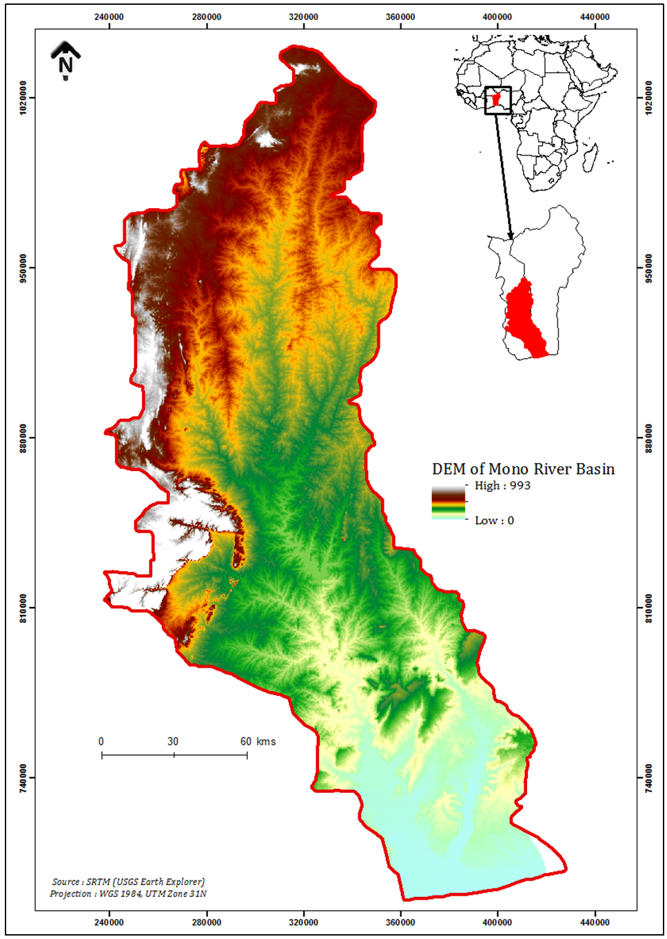Figure 1. Study area Location

2.2. The Paper Should Have the Following Structure

Graphic analysis is a technique that helps highlight certain explanatory factors in the correlation and dependence between some retained variables. It starts from the data obtained and is based on some observation logics [16]. The explorator, thanks to a very well furnished toolbox, will have the opportunity to observe the information all over, with a tentative to highlight the different structures, and, if applicable, to formulate possible assumptions. The explorator will not focus on any « optimality » of the tool used, and the fact of understanding that the latter behaves « well » in most situations, is just enough [28]. Climate parameters such as rainfall, temperature, at annual, monthly, decennial and inter-annual scales, are very often exploited [7]. Such method consists in representing the histograms (or graphs) of all the observations along with the trends that help to restrict their evolution visually during the period of study. An objective and rigorous interpretation of the results helps obtain a global vision and identify possible form of irregularity [7].

2.3. Analysis Related to Evidences

2.3.1. Nicholson Index

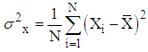
The Nicholson index is used to examine rainfalls interannual evolution and the nature of the tendency [29]. It is a simple, powerful and flexible tool based at the same time on meteorological data, and allows to stress the surplus and and deficit periods within the same chronological series [30, 31]. It gives the advantage of determining the hydric deficit at the scale of the various seasons and the year at the same time [32]. The choice of that index is justified by its capacity to rapidly detect situations of drought and assess their acuteness. It is also highly recommended by climatologists due to the fact that it is less complex than many others, notably the Palmer drought index. The Nicholson index is expressed by the equation (1) [33].

(1)

Where: the average rainfall; the standard deviation, X_i : rainfall of the year and i.

A normal period is a period during which, the annual rainfall is sensibly equal to the average annual rainfall, i.e., the index value is equal to zero [34]. Period is wet, when the index value is positive, i.e. the annual rainfall is higher than the average; period is dry when the index value is negative, i.e., annual rainfall is less than average [35].

2.3.2. Monthly Rainfall Index

The monthly rainfall coefficient helps represent the distribution, in terms of percentage, of monthly rainfalls during the year. It permits to set up some division of the year in order to determine the rainy period (the most watered months) and estivale (the least watered months) [36]. It is defined by the monthly values ratio on the chronical average given by equation (2) [37].

(2)

P_i: average monthly rainfall; interannual module

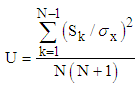
2.4. Research of Potential Ruptures

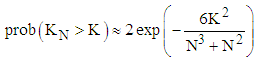
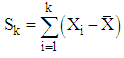
A break in the time series can be generally defined as an abrupt change in the probability law of the series at a given time, usually unknown. It corresponds to a trend reversal of the time series [4]. In this article, we focused on the break detection tests of Pettitt t, Buishand and Hubert. Forall these tests, the null hypothesis that must be tested is H₀ « no break in the series » [38]. The choice of these tests is justified by their foundation, power, robustness, and success for such a study throughout the world [39, 40].

ü Pettitt test

The Pettitt approach is non-parametric and is derived from the Mann-Whitney test. The absence of break in the series (xi) of size N is the null hypothesis. The use of the test supposes that for any time t with a value between 1 and N, the two time series (Xi) for i = 1 to t and for i = t + 1 to N belong to the same population. The variable that is to be tested is K_N, the maximum in absolute terms of the variable U_t,N defined by the relation (3) [41, 42]:

(3)

Where D_i,j is the coefficient given by equation (4)

(4)

If k is the value of K_N taken on the studied series, under the null hypothesis, then the probability of exceeding of the value k is given approximately by equation (5) [43]:

(5)

If Prob (K >k ) < α , for a significance level α, then the null hypothesis is rejected, then an estimation of the date of the break is provided by the moment t defining the maximum in absolute terms of the U_t,N variable.

ü Buishand test

The Buishand procedure refers to the same model and to the same hypotheses as the Lee and Heghinian approach. If the assumption is that there is a uniform distribution for the position of the break point t, the Buishand U statistic is defined by equation (6) [29]:

(6)

Where the terms S_k and σ_x are respectively partial sum and standard deviation given respectively by equations (7) and (8):

(7)

(8)

The null hypothesis of the statistical test is the absence of break in the series. In the case of rejection of the null hypothesis, no estimation of the date of the break is proposed by this test. In addition to these different procedures, the building of a control ellipse makes it possible to analyze the homogeneity of the (xi) series. Under the null hypothesis assumption, the SA variable, defined above, follows a normal distribution with a zero mean and a variance equal to equation (9) [44]:

(9)

With, k = 0 to N.

This control ellipse was used here to estimate visually the importance of the deviations under the null hypothesis of the homogeneity of the series. It is consequently possible to define confidence limits including the series of the S_k.

ü Hubert test

Hubert’s segmentation procedure detects the multiple breaks in time series. The principle is to cut the series into m segments (m>1) such that the calculated means of the neighboring sub-series significantly differ. To limit the segmentation, the means of two contiguous segments must be different to the point of satisfying Scheffe’s test [45]. The procedure gives the timing of the shifts. Giving a m^thorder segmentation of the time series, i_kk = 1,.m, the rank in the initial series of extreme end of the k^th segment (with i₀= 0), the following are defined by equation (10) [46]:

(10)

D_mis the quadratic deviation between the series and the segmentation given by equation (11)

(11)

For a given segmentation order, the algorithm determine the optimal segmentation of a series that is such that the deviation D_m is minimal. This procedure can also be interpreted as a stationary test, the null hypothesis being the studied series is non-stationary. If the procedure doesn’t produce acceptable segmentations of order bigger or equal to two, the null hypothesis is accepted [45].

2.5. Application

This study deals with the Mono-Couffo watershed, notably in its low valley, in Benin. It is based on rainfalll data collected from the Cotonou station during a period extending from 1953 to 2014. Our procedure is essentially structured in 3 components: a component related to the explanatory analysis, a component related to the indexes and a component related to the statistical processing. At that level, our motivation is to identify the different extreme situations the Mono area had to face during that chronical, and also to extract all necessary information that could help inform the climate characteristics of that period.

ü In component 1

At annual scale, we have exploited the annual rainfalls, in parallel with the average, in order to visualize the rainy and dry years. We have subsequently calculated the rainfall averages for humid years (noted SYA) and the averages of dry years (noted DYA); such action helps identify the very humid years and the very dry ones. In the same line, we have exploited the annual amplitudes, as compared to the average, in order to identify the years that had strong amplitudes and weak amplitudes; we have then calculated the rainfall averages for strong amplitude years (noted SYAA) and the averages of weak amplituude years (noted DYAA), in view of identifying the very strong and very weak amplitudes. In the same event, at monthly scale, we have equally exploited all monthly rainfalls in order to identify on the one hand, the months that were very humid, humid, dry, and very dry, and on the other hand, the months with amplitudes that were very strong, strong, weak and very weak.

ü In component 2

As for indexes, we have calculated the Nicholson index and then proceded to its exploitation as opposed to the reference value (zero), all this to help highlight the deficit and excess years. Afterwards, the index average for the deficit years is calculated (noted, DYIA) and for the excess years (noted, SYIA), the point is to detect the very excedentary and very deficient years. In the same way, the rainfall monthly index is evaluated as compared to the average in order to visualize the winter seasons (the most watered months) and summer months (the least watered seasons).

ü In component 3

In the statistical process, we have applied the Pettitt Pettitt, Hubert and Buishand tests in order to asssess the heterogeneous or homogeneous character of the series thanks to the Khronostat software used to that effect. In events where the series are heterogenous, the rupture year and its direction altogether will be specified. The monthly data of that year are exploited with the same tests in order tro search for the month that corresponds to that rupture.

As regards the two first components, the philosophy adopted is presented as follows: A year is considered as deficit when rainfall is inferior to the average and excedentary when the average is erexceded. A highly defict year is a year that has received rainfall inferior to the average of deficit years and a very excedentary year is a year that has received rainfalls superior to the average of excedentary years. We have applied the same philosophy as much for the annual amplitudes as for the monthly ones. The totality of the results is presented in the form of tables and graphs.

3. Results and Discussion

3.1. Results Related to Graphic Analysis

3.1.1. Annual Scale

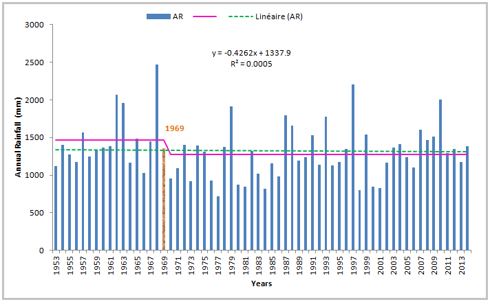
Figure 2a presents the annual rainfalls contributions during the period extending from 1953 to 2014 as opposed to the average results and figure.2.b compares DYA and SYA. The analysis of figure 2.b shows that over the 62 years covering the period studied, 32 years have been dry with 30 humid ones. The analysis of the figure shows 9 years that were noticeably very humid and 13 others plainly very dry. The maximum (2470.2) is observed in 1968 and the minimum (719.4) in 1977. The gap between the maximum and the minimum (551.1mm) reached 1750.8 mm, a fact that explains the wide annual rainfall contrast monitored from the Cotonou station. Figure 2c represents the synthesis of figures 2a and 2b. Its observation helps in the organization of rainfall measures in the Cotonou station under four distinct categories: very humid years (a), humid years (b), very dry years (d) and dry years (c) as illustrated in figure 2c. As a result, the temporal variation of annual rainfalls shows that the annual regime is very irregular from one year to the other.

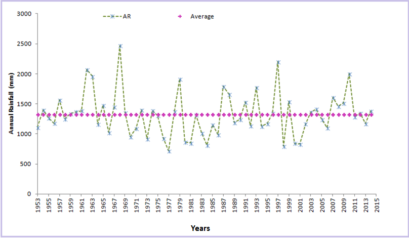Figure 2a. Identification of humid and dry years over the 1953-2014 period

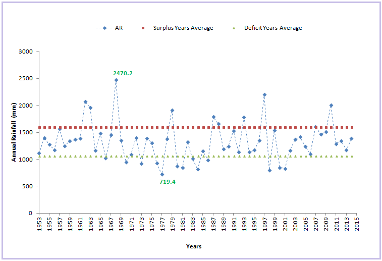Figure 2b. Identification of humid years and dry years over the 1953-2014 period

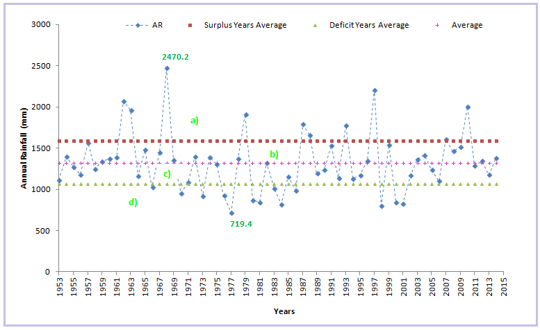Figure 2c. Organization of Cotonou’s annual rainfall from 1953 through 2014

ü Annual amplitudes distribution

Figure 3a represents the annual amplitudes distribution on the period covered by the study in relation with the average and figure 3.b deals with the distribution compared to the limits previously defined. The analysis of this figure provides 30 years of strong amplitudes and 32 of weak amplitudes. The analysis of figure 3.b indicates 9 years of very strong amplitudes and 13 years of very strong amplitudes. The maximum amplitude is located in 1962 and the minimal one in 1984. The gap between the maximum (833.7mm) and the minimum (157.8mm) is equal to 675.9 mm; such information is related to the annual rainfall amplitudes contrast oberved in the Cotonou station. Figure 3c is the synthesis of figures 3a and 3b. The analysis of figure 3c helps to sort out annual amplitudes into four categories: very strong amplitudes (a), strong amplitudes (b), very weak amplitudes (d) and weak amplitudes (c) such as represented by figure 3c.

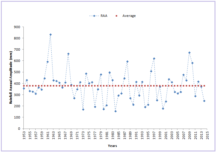Figure 3a. Identification of years with strong and weak amplitudes during the 1953-2014 period

Figure 3b. Identification of years with very strong and very weak amplitudes over the 1953-2014 period

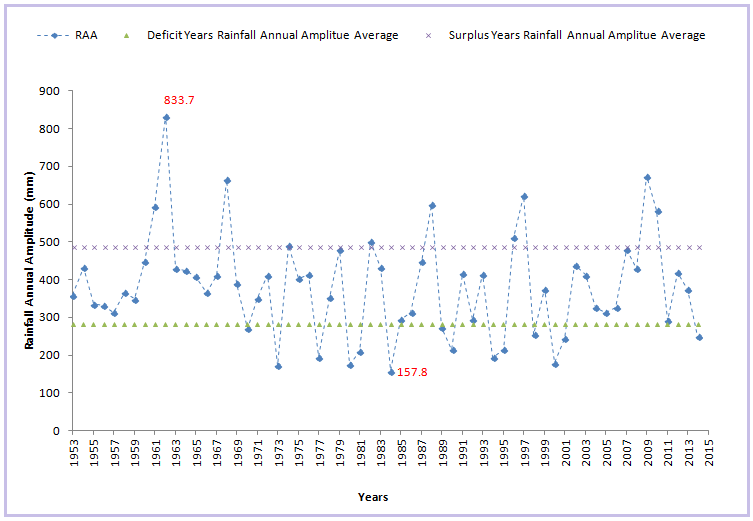
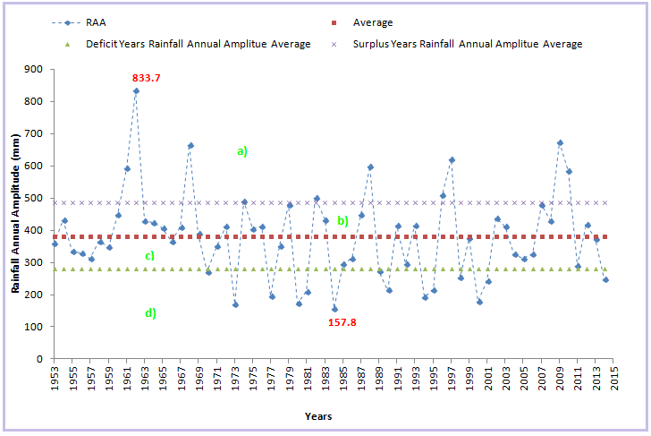Figure 3c. Organisation of annual rainfall amplitude in Cotonou from 1953 through 2014

3.1.2. Monthly Scale

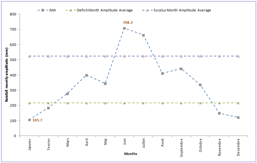
ü Monthly rainfalls distribution

We will present in figure 4a rainfall distribution on a monthly scale in parallel with the average and figure.4b in relation with (DMA, SMA), in the Mono watershed in the Cotonou station. The purpose is to better understand the temporal distribution of the Mono watershed outlets. The analysis of figure 4a reveals 5 surplus months (April-May-June-July-October) and 7 deficit months (January, February, March, August, September, November and December). The analysis of figure 4b, places May and June in the months with very heavy rainfall and December and January the months with very weak rainfall. The difference between the maximum (349.8mm) and the minimum (16.0mm) reaches 333.8 mm. This highlights two distinct phases for the months which present some visible contrast in terms of rainfalls.

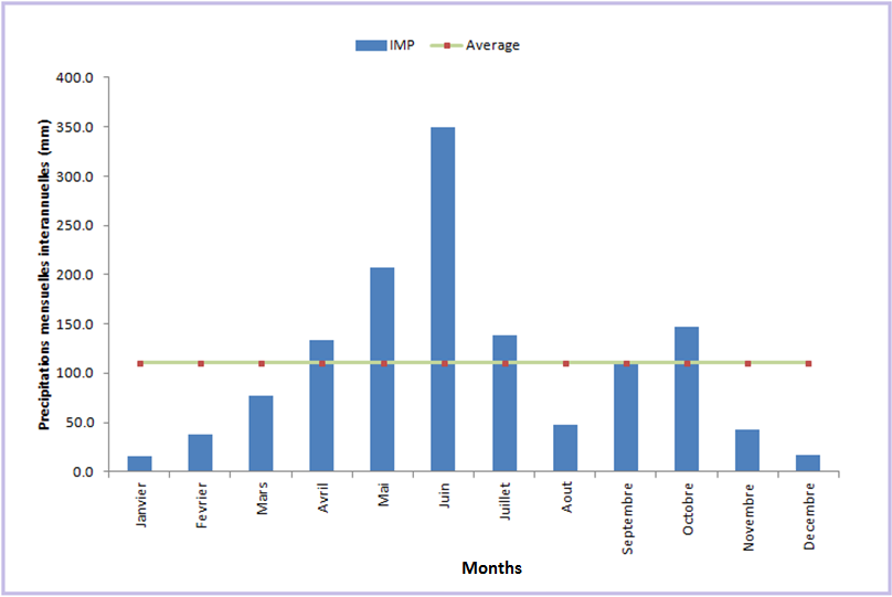Figure 4a. Identification of surplus and deficit months between 1953 and 2014

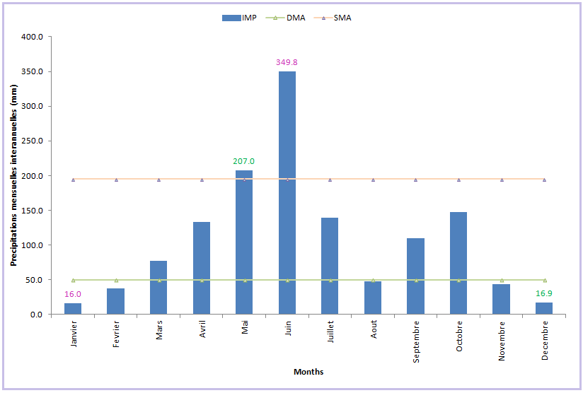Figure 4b. Identification of very excedentary and very deficit months from 1953 to 2014

ü Monthly amplitude distribution

Figure 5a presents the monthly amplitudes distribution of the period covered by the study in relation with the averages and figure 5.b the distribution established in compliance with the limits already defined. The analysis of figure 5a shows 4 months with strong amplitudes (April, June, July, August and September, 6 months with weak amplitudes (November, December, January, February and March) and 2 months with regular amplitudes (May-October. The maximal amplitude is situated in June and the minimal one in January. The gap between the maximum (708.3mm) and the minimum (105.7mm) is equal to 602.6 mm; this clearly shows the contrast of rainfall amplitudes in the Cotonou station.

Figure 5a. Identification of months with strong and weak from 1953 to 2014

Figure 5b. Identification of months with very strong and very weak amplitudes from 1953 to 2014

3.2. Results Related to Indexes

3.2.1. Monthly Rainfall Index

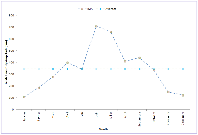
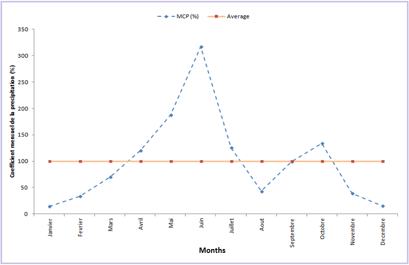
Figure 6 illustrates the distribution index of monthly rainfalls in the Mono watershed at the Cotonou station. The analysis of the figure reveals two rainy seasons (the most watered): mid-March to mid-July corresponding to the extensive rainy season; mid-September to mid-October corresponding to the short rainy season and two summer seasons (the least watered months): .mid-October to mid-march corresponding to the extensive dry season and from mid-July to mid-September corresponding to the short dry season.

Figure 6. Rainfall seasonal distribution at the Cotonou station

3.2.2. Nicholson Index

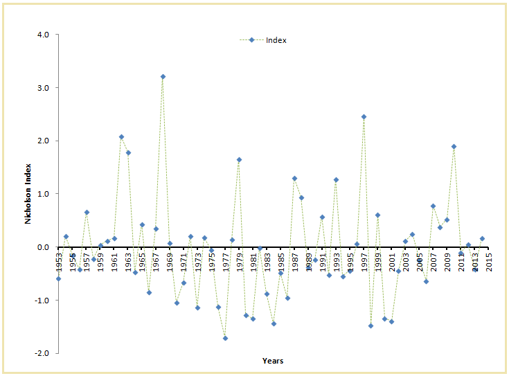
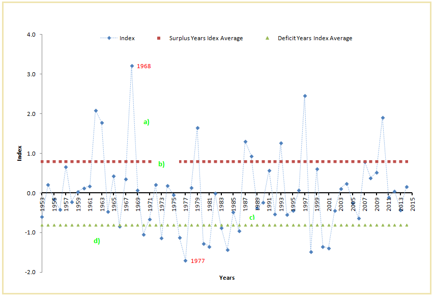
Fugure 7a represents the Nocholson index distribution in relation with the reference and with figure 6b established in comparison with the limits defined. The point is to set up some punctual analysis of the annual rainfall variations in Cotonou. The analysis of figure 7a reveals 30 dry years, 29 humid years and 3 normal or regular years. The analysis of figure7b in relation with the superior and inferior limit, allowed the identification of 9 very humid years and 12 very dry years. Considering the zero reference value, figure 7b highlights four different categories of years in terms of rainfall (very humid (a), humid (b), very dry (d) and dry (c). 1968 stands as the rainiest year and 1977 the least rainy one. This accurately confirms all previous results. Globally, these results show that the deficit periods slightly extend in space while being a little bit more persisting in time than the surplus periods.

Figure 7a. Identification of dry and humid years during1953-2014

Figure 7b. Organisation of annual rainfall at the Cotonou station during 1953-2014

3.3. Results Related the Rupture Detection

3.3.1. Annual scale

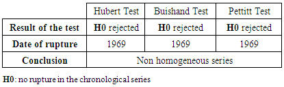
The table below presents the results of the rupture tests. Figures 8a, 8b and 8c are respectively related to the Hubert, Buishand and Pettitt tests. The results are therefore more reliable. All tests reject the null hypothesis of an lack of rupture at level 95%. The date of that rupture is provided by the Buishand ellipse (figure 8b) and corresponds to years 1969. The Hubert (figure 8a) and Pettitt tests (figure 8c) confirm this result, while proposing anew the date of 1969 as a year of rupture. The direction of that rupture provides a general decrease trend (figure 8a). The consistency of those results allows the following conclusion: the Cotonou chronological series is not homogeneous and can therefore be divided into two sub-series: 1953-1969 and 1970-2014.

Table 1. Tabular results of breaking test

Figure 8a. Hubert segmentation diagram at the annual scale

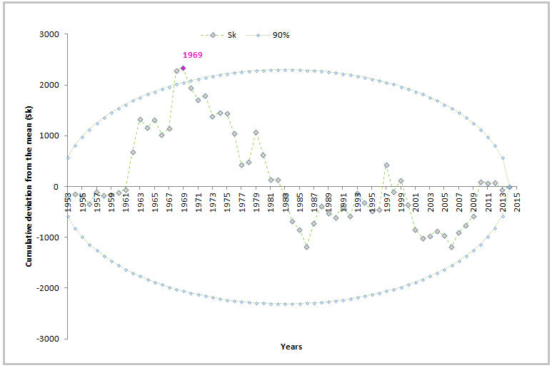Figure 8b. Control ellipse of Buishand

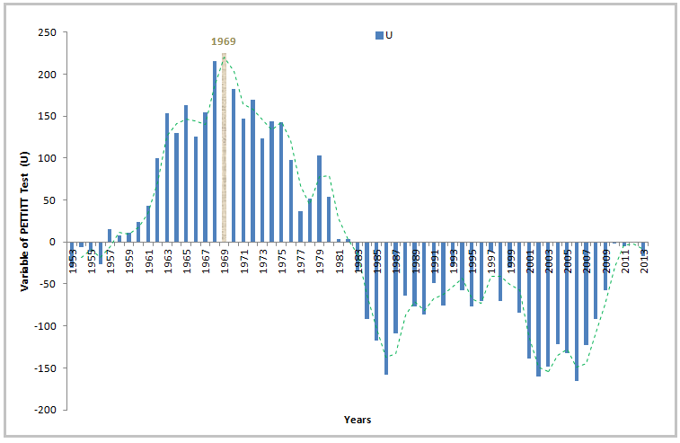Figure 8c. Pettitt variable diagram

3.3.2. Annual Scale

Figure 9 represents the Hubert segmentation related to the monthly data collected in year 1969, which corresponds to the year of rupture. The point here is, subsequent to the identification of the rupture date at the annual scale with the three tests, to detect the month that best corresponds to that rupture. We will here exclusively focus on the Hubert test. As we can notice, there is some rupture in the month of October and the trend curb shows general tendency to decrease. As a result, the rainfall series studied in the current article is related to a rupture in decrase in October 1969. This result confirms the drought Sub-Saharan Africa had to face in the years 1960-1970.

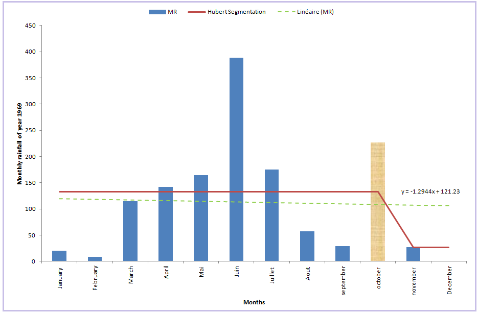Figure 9. Hubert segmentation diagram related to 1969 year

4. Conclusions

The current article deals with the Mono-Couffo watershed, notably in its low valley, in Benin. It is based on rainfall data collected from Cotonou and covers the period 1953-2014. The objective targetted here is, on the one hand, the identification of the different climate situations and characteristics of the zone of study during that chronical and, on the other hand, the emphasis of the general rainfall distribution (trends, variability, extremes, etc.), the dry-humid shifts and the evaluation of their space and time amplitude; such information constitute key elements for any reflection related to the fight against climate change. In order to reach this objective, we have initially undertaken a graphic analysis based on some observations; annual and monthly rainfalls, annual and monthly amplitudes have been exploited to that effect. We have subsequently proceded to the calculation of all rainfall-related indexes; the Nicholson index and the monthly rainfall index have also been exploited. We have eventually undertaken a statistical data processing; in that regard, the rupture detection tests (Pettitt, Hubert and Buishand) have been implemented with the use of the Khronostat software. The results obtained are globally reliable. As for the annual scale, the results show an alternance of humid and dry periods along with an organization of rainfall in Cotonou under four different year categories: very humid, humid, very dry and dry. The maximum is situated in 1968 and the minimum in 1977. In the same perspective, the results related annual amplitudes show four amplitude categories: very strong, strong, very weak and weak; the maximal amplitude is situated in 1962 and the minimal one in 1984. As for the monthly scale, the results reveal 5 surplus months (April, May, June, July, October) and 7 deficit months (January, February, March, August, September, November and December). June stands as a month with very heavy rainfall and January, as the month with very low rainfall. In the same line, as regards monthly amplitudes, the results provide 4 months with wide amplitudes (April, June, July, August and September), 6 months with very weak amplitudes (November, December, January, February and March) and 2 months with regular amplitudes (May-October). The maximal amplitude is observed in June and the minimal one in January. Concerning the indexes calcualted, the monthly rainfall index revaels two winter seasons (among the most watered ones): mid-March to mid-July corresponding to the extensive rainy season; mid-September to mid-October corresponding to the short rainy season and two summer seasons (the least watered ones): .mid-October to mid-march corresponding to the extensive dry season and mid-July to mid-September corresponding to the short dry season. The Nocholson index for its part helps identify 9 very humid years and 2 very dry other ones. Futhermore, it contributes to the establishment of 4 distinct categories in terms of rainfall: very humid, humid, very dry and dry. 1968 is again the most rainy year and 1977 the least rainy one. This accurately complies with the result previously obtained. Finally as regards the statistical study, the different tests reject the series consistency and corroborate with 1969 as the same rupture date, more precisely in the month of October. Ultimately, rainfall in Cotonou has been subject to irregularity and some general tendency to decrease; in fact, the deficit periods are slightly more extended in space and a little bit more persisting in time than the surplus periods. Such results provide some very interesting indications for climate experts and specialists, notably in the relations with the phenomena that contribute to the fight against global warming. However, it would be more convenient to combine the data collected by the specialized services on the field, including the ones that have been considered in the current study, with those obtained by satellite observations, in order to establish some parallel with ground rainfall spatial structure and those of the altitude collection convective systems. This will further contribute to the constitution of tools that facilitate very performing decision-making processes for emerency programmes.