-
Paper Information
- Next Paper
- Paper Submission
-
Journal Information
- About This Journal
- Editorial Board
- Current Issue
- Archive
- Author Guidelines
- Contact Us
Resources and Environment
p-ISSN: 2163-2618 e-ISSN: 2163-2634
2014; 4(3): 115-138
doi:10.5923/j.re.20140403.01
Estimating Plume Emission Rate and Dispersion Pattern from a Cement Plant at Yandev, Central Nigeria
 Abstract
 Reference
 Full-Text PDF
 Full-text HTML
Fanan Ujoh1, Olarewaju O. Ifatimehin2, Isa D. Kwabe3
1Department of Urban and Regional Planning, Benue State University, Makurdi, Nigeria
2Department of Geography and Planning, Kogi State University, Anyigba, Nigeria
3Federal Character Commission, Abuja, Nigeria
Correspondence to: Olarewaju O. Ifatimehin, Department of Geography and Planning, Kogi State University, Anyigba, Nigeria.
| Email: |  |
Copyright © 2014 Scientific & Academic Publishing. All Rights Reserved.
Cement production at Yandev, Nigeria commenced in 1980 without an environmental impact assessment to ascertain the extent of damage production activities would bring to bear on the physical conditions of the host environment. This study was carried out to provide baseline data on the rate and pattern of plume rise from the factory. Field survey was employed for primary data collation, while secondary data (climatic and factory data) were acquired from NIMET Makurdi Office and Dangote Cement Plc. Plume rate was estimated using the Gaussian (Mathematical) Model; Kriging, using Arc GIS, was adopted for modelling the pattern of plume dispersion. ANOVA and HSD’s Tukey test were applied for statistical analysis of the plume coefficients. The results indicate that plume dispersion is generally high with highest values recorded for the atmospheric stability classes A and B, while the least values are recorded for the atmospheric stability classes F and E. The variograms derived from the Kriging (spatial correlational analysis) reveal that the pattern of plume dispersion is outwardly radial and omni-directional. With the exception of 3 stability sub-classes (DH, EH and FH) out of a total of 12, the 24-hour average of particulate matters (PM10 and PM2.5) within the study area is outrageously higher (highest value at 21392.3) than the average safety limit of 150 μg/m3 - 230 μg/m3 prescribed by the 2006 WHO guidelines. This indicates the presence of respirable and non-respirable pollutants that create poor ambient air quality. The study concludes that the environmental compliance status of Dangote Cement Plc, Yandev towards attaining sustainability for the host communities and physical environment is far from meeting the target requirement as spelt by the Millennium Development Goals No. 7. The study recommends ameliorative measures including periodic environmental audits; and adoption of technologies that would reduce the rate of plume emission.
Keywords: Plume dispersion coefficients, Spatial autocorrelation, Gaussian model, Yandev- Nigeria
Cite this paper: Fanan Ujoh, Olarewaju O. Ifatimehin, Isa D. Kwabe, Estimating Plume Emission Rate and Dispersion Pattern from a Cement Plant at Yandev, Central Nigeria, Resources and Environment, Vol. 4 No. 3, 2014, pp. 115-138. doi: 10.5923/j.re.20140403.01.
Article Outline
1. Introduction
- Global attention is now focused on declining quality of the environment resulting from the rapid expansion in resources exploitation. There is an increasing need to use resources in a sustainable way, such that there is concurrent increase in production while also protecting the environment, biodiversity, and global climate systems. This type of compromise requires careful resource planning and decision-making at all levels [1].Nigeria’s environment (at urban and rural levels) has suffered an accelerated decline in quality of air, soils, biodiversity and water resources [2-12]. It is clear that sound natural resources management and planning are essential to tackling the aforementioned problems and to promote sustainable development.Mining activities represent human actions that cut through the landscape, scarring and interfering with the natural habitat conditions as well as micro-climatic conditions [13]. Specifically, the environmental effects of limestone mining and cement production are known to impoverish the flora and fauna of host environment, result in sediments deposition in riverine systems, create large mining spoil mounds and deep mining lakes, result in loss of timber resources and other vegetal cover, toxification and pollution due to chemical wastes or weathering of mining spoils, cause changes in micro-climate, and several others. These effects on the ecosystem are not only on-site but also occur off-site as well. These, in turn, significantly alter the environmental spheres of the affected areas. The significance of this study is premised on the fact that limestone exploitation and cement production commenced at the study area prior to the promulgation of Nigeria’s environmental impact assessment (EIA) Decree 86 of 1992, implying that no EIA was conducted at the study area. In addition, among the human activities that pose the highest threat to the conservation of biodiversity and fragile ecosystems (thereby promoting environmental degradation) is mining of mineral resources, including limestone. Additionally, findings from a recent study on cement plume rise and dispersion rate at the study area [14] reveal high concentration of pollutants from plume.Presently, construction work has commenced on a second cement manufacturing plant at ‘Mbatiav’, within the same Local Government Area (LGA). Considering the observed environmental impact of the present cement plant, there is need to carry out a some form of assessment of the extent of damage on the host environment as a step in the direction of impact mitigation for the present facility; and prevention for future/proposed facilities. This is necessary as we hope to develop a system of resource exploitation that would not compromise the ability of future generations to cater for their needs.This study assesses the status of plume rise, dispersion and concentration rates within the study area.
2. Materials and Methods
2.1. Study Area
2.1.1. Brief History and Location
- The cement factory is located at Yandev, near Gboko town, in Gboko LGA of Benue State in Nigeria. Gboko LGA is located between Latitudes 07º 08ʹ 16ʺ and 07º 31ʹ 58ʺ, and Longitudes 08º 37ʹ 46ʺ and 09º 10ʹ 31ʺ. The central location of the factory is at 7º 24ʹ 42.45ʺN and 8º 58ʹ 31.28ʺE, at about 532 feet above mean sea level (Figure 1 and Plate 1).
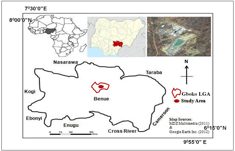 | Figure 1. Locational Map of Study Area |
2.1.2. Climate
- The study area is located within a sub-humid tropical region with mean annual temperature ranging from 23ºC to 34ºC, and is characterized by two distinct seasons: the dry season and rainy season. The mean annua1 precipitation is about 1,370mm [15], with an average wind speed of 1.50 m/s [16].
2.1.3. Geology and Drainage
- The study area is located within the general area of the Benue Trough, which is largely covered by Cretaceous continental and marine sediments [17] (see Figure 2). The Benue floodplain is filled with Quaternary heterogeneous sediments [18], while its geology is a combination of the pre-cambrian basement formation comprising the lower and upper cretaceous sediments, in addition to some volcanic deposits [19]. The resources are grouped into Pre-cambrian limestones, marbles and dolomites, Cretaceous and Tertiary limestones, as well as concretionary calcretes. However, the reserves at Yandev (the study area) are of Cretaceous formation and in excess of 70 million tonnes [20-22].
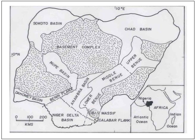 | Figure 2. Geological Map of Study Area |
2.1.4. Soils and Vegetation
- The soils of the study area are classified as Acrisols (Ortic and Ferric subgroups) and Dystric Cambisols [18]. The well drained soils have predominantly low activity clay fractions (kandic property), low to medium base status and low water and nutrient retaining capacities like most other upland soils of the sub-humid region [23]. The soils are generally agriculturally rich and support high cereals and tuber produce. Naturally, the vegetation of the area was dominated by southern guinea savannah type, although at present, extensive cultivation, annual bush-burning, limestone mining and several other anthropogenic activities have transformed the vegetation into shrubs and bushes (Figure 3).
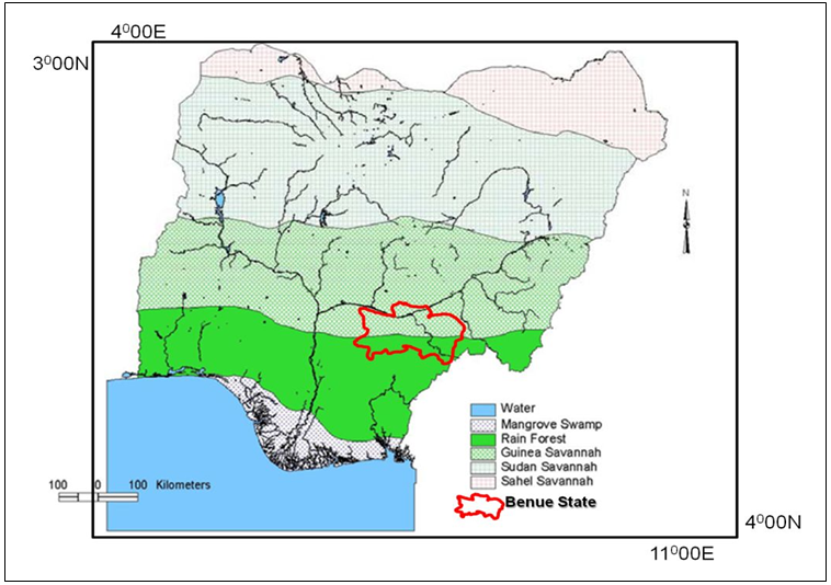 | Figure 3. Vegetation Map of Study Area |
2.1.5. Population and Economy
- The population of Gboko LGA is 358,936 [24], and is largely pre-occupied in subsistence agriculture and hunting. The study area is ancestral home to the Tiv, presumably the 4th largest ethnic group in Nigeria. However, with the establishment of cement production, a ‘settler’ population is expanding to provide various economic services for the business community at the factory. The most prominent communities within the study area are Tse-Kucha and Tse-Amua with proximity to the factory of distance of 1.8 km and 3.07 km, respectively from the factory.
2.2. The Point Source Gaussian Model
- The Point Source Gaussian Model (also called the Mathematical Model) was applied by [14] for a similar study (using data up to the year 2006). The model provides for the determination of cement dust concentration (in μg/m3) from cement plants using the point source plume function given below as;
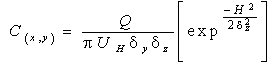 | (1) |
2.2.1. Field Survey
- On-site, primary data for the study was obtained through the use of a hand-held GPS unit and photographs using a Nikon Camera. Also, field surveys were conducted to collect the pre-requisite data employed for generating estimates of plume dispersion coefficients and the consequent dispersion patterns. Secondary data was collected from various sources (see Appendix 1).
2.2.2. Software
- ArcGIS 9.3 and SPSS software were used for data processing and statistical analysis.
2.2.3. Atmospheric Stability Classes Definition
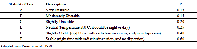
- The determinants of the stability classes are wind speed and temperature (state of insolation and irradiation). These together affect the lapse rate, the absence or presence of convective activity, and the dynamics of the mixed layer as explained by [27]. Six atmospheric stability classes were adopted for this study (see Table 1). Classes A, B and C are conditions prevalent during daytime; D could be obtainable during daytime (under heavy cloud conditions) or at night; while E and F are mainly night time conditions [28; 29]. Table 2 provides in-depth explanation regarding the prevailing condition and time of the day.
|
|
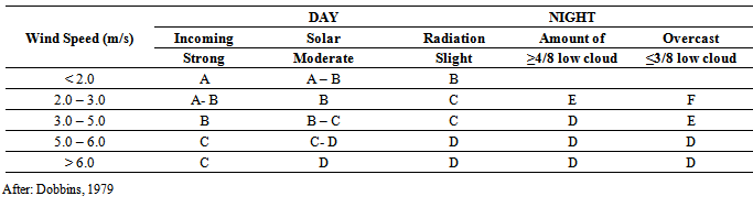
- The provisions on Table 2 imply that:● Strong solar radiation corresponds to a solar elevation angle 600 or more, above the horizon;● Moderate solar radiation corresponds to a solar elevation angle of between 350 – 600;● Slight insolation corresponds to a solar elevation of 150 – 350;● For A-B, B-C, or C-D conditions, average values are computed for each class.
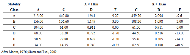
2.2.4. Calculating the Dispersion Coefficients
- Based on vertical and horizontal downwind dispersion coefficients, the algebraic representation of the dispersion coefficients using Table 4 is frequently expressed in terms of Power Law expression of the type:
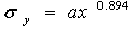 | (2) |
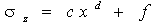 | (3) |
|
|
 is a linear combination that may be written as:
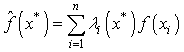 | (4) |
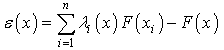 | (5) |
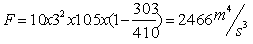
2.2.5. Determination of Buoyancy Flux Parameters
- Observation of plume emitted from a stack at a temperature Ts above the ambient air temperature Ta shows that the plume rises above the top of the stack due to several factors prominent among which are thermal buoyancy, momentum of the exhaust gases, and the stability of the atmosphere. Hence, as described by [14], buoyancy results when exhaust gases are hotter than the ambient air, or when the molecular weight of the exhaust gas is lower than that of air (or a combination of both factors). Momentum is caused by the mass and velocity of the gases as they leave the stack. The buoyancy flux parameter (F) was determined prior to the calculation of the plume rise. The function for deriving the buoyancy flux parameter (F) is given as:
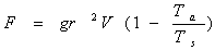 | (6) |
 | (7) |
2.2.6. Statistical Analyses
- Three statistical data analysis techniques were engaged to test the estimated plume dispersion coefficients. These are descriptive statistics, analysis of variance (ANOVA), and post-hoc multiple comparisons.
3. Results
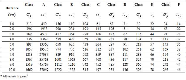
3.1. Plume Dispersion Coefficients
- The plume dispersion coefficients for the study area (Table 4) were calculated using the constant values in Table 3. Vertical (z) and horizontal (y) dispersion coefficient modelling was done for a distance of 1 – 10 kilometers for all atmospheric stability classes (A – F). The results show that Class ‘A’ is the most unstable class followed by Class ‘B’. Hence, they have recorded the highest and second highest values of plume dispersion coefficients, respectively. Class ‘F’ exhibits the least values and is considered the most stable class.
3.2. Statistical Analysis of Plume Dispersion Coefficients
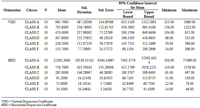
- Statistical analyses were conducted to test the extent of variation of the plume dispersal coefficient values between the six atmospheric stability classes (A, B, C, D, E and F). Table 5 shows that for the Vertical Dispersion Coefficient (VDC), the highest and lowest mean values are recorded from Classes A and F, respectively, while for the Horizontal Dispersion Coefficient (HDC), the highest and lowest mean values are recorded from Classes A and B, respectively. Extreme variation in the standard deviation, standard error and minimum and maximum values of all 6 atmospheric stability classes was also observed, but could be explained as a function of prevailing weather conditions and time of the day which together are determining factors controlling the pattern of plume dispersion and eventual rate of deposition at various points within the study area.
|
|
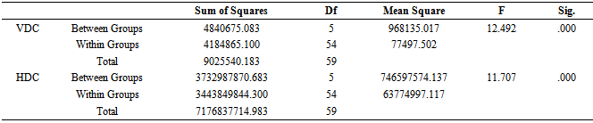
- The analysis of variance (ANOVA) result (Table 6) is the key table because it shows whether the overall F ratio for the ANOVA is significant. The ANOVA F-distribution function is used to determine how significantly variable the data from the atmospheric stability classes are. The goal is to test if plume dispersion results for the 6 atmospheric stability classes are equal (or otherwise), i.e., whether; VDC = HDC = 0. The ANOVA results reveal significant variation in the mean values of plume dispersion between and within the stability classes for both VDC and HDC orientations. This is because the probability distributions of VDC and HDC (0.000) all fall below the critical level value of 0.05 set for ANOVA. Since the ANOVA results are found to be significant using the above procedure, it implies that the values of the means differ more than would be expected by chance alone. The variation in the ANOVA results requires further detailed analysis to identify the nature of variation between the values of the means of the atmospheric stability classes. To address this, the post hoc test is applied (see Appendix 2). Values for Tukey’s HSD (honestly significant difference) and Fisher’s LSD (least significant difference) contains a high level of redundancy, nevertheless some key discoveries are made as specific mean values under specific atmospheric stability classes are found significant at the 0.05 alpha level. These have been flagged.
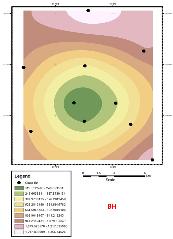
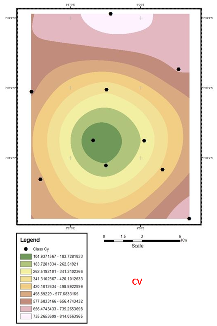
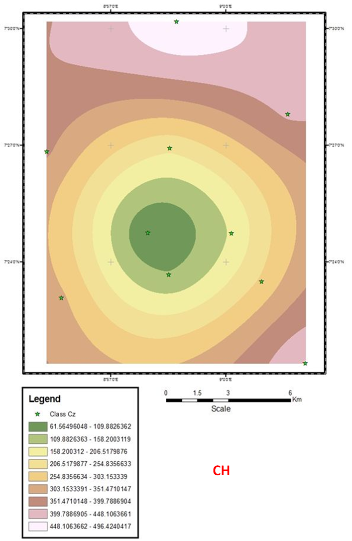
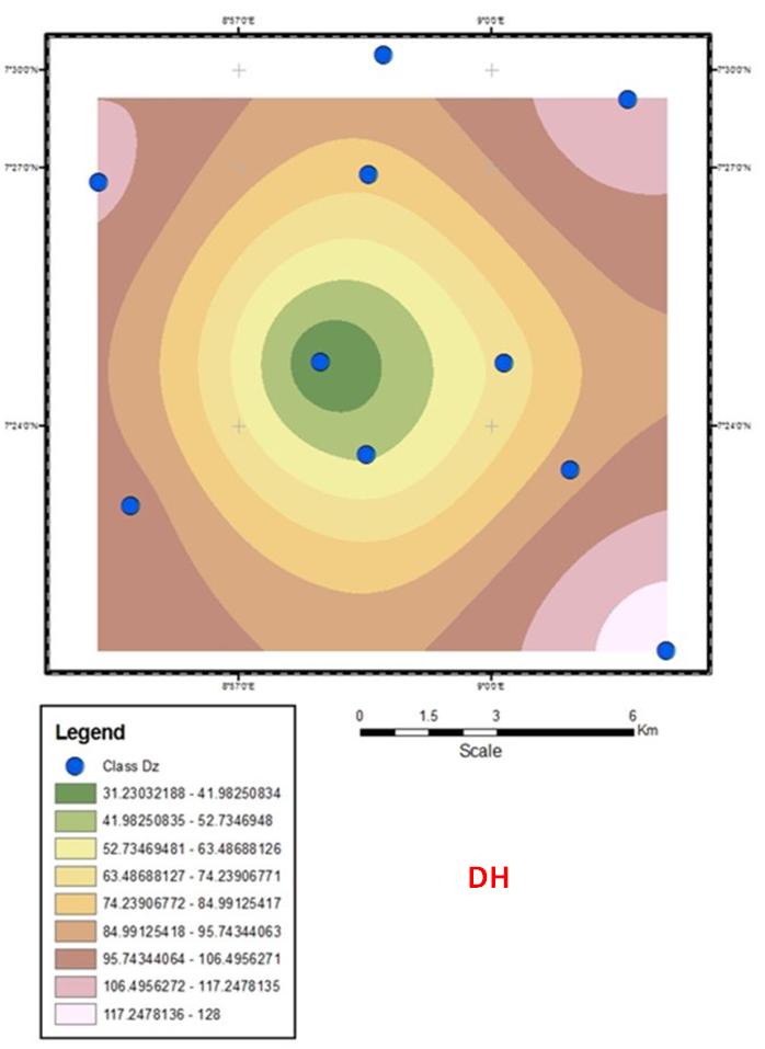
3.3. Spatial Autocorrelation of Plume Dispersion Coefficients
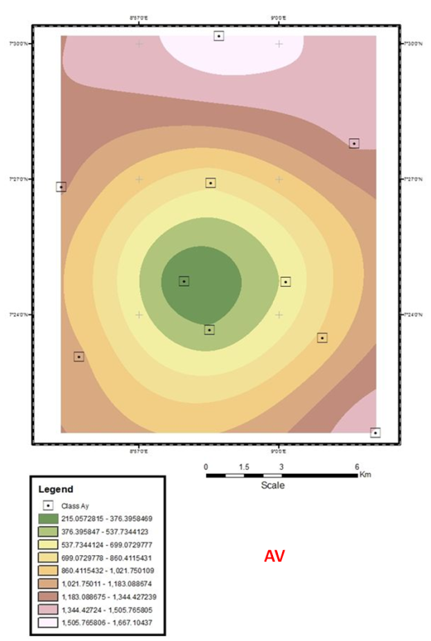
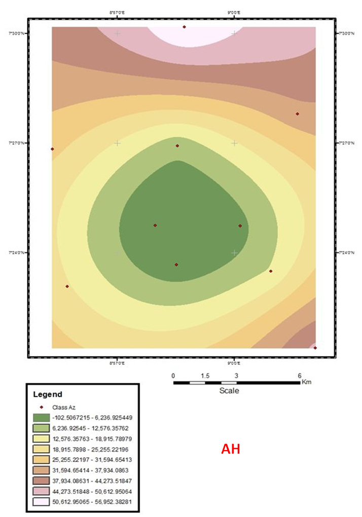
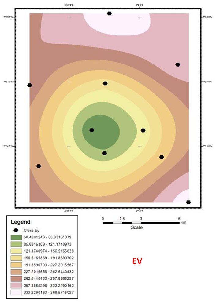
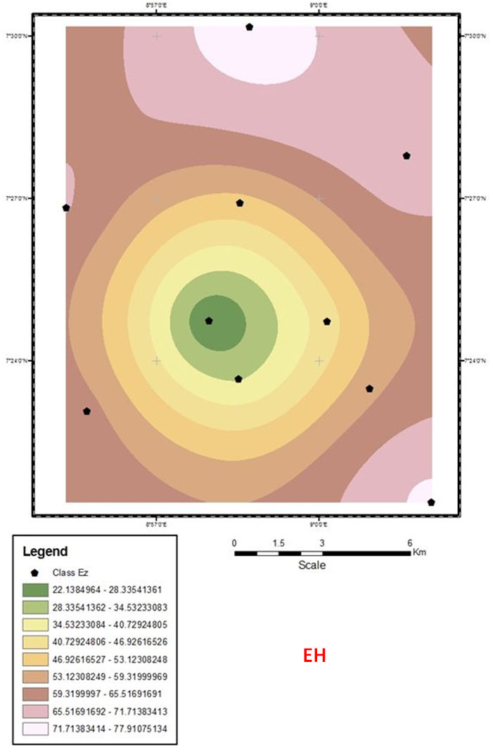
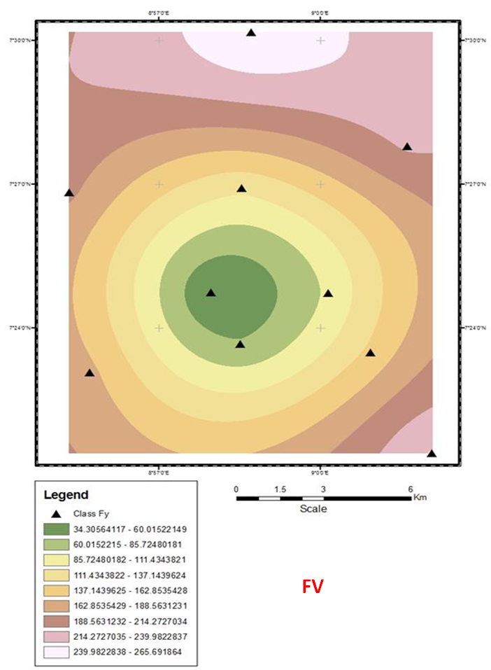
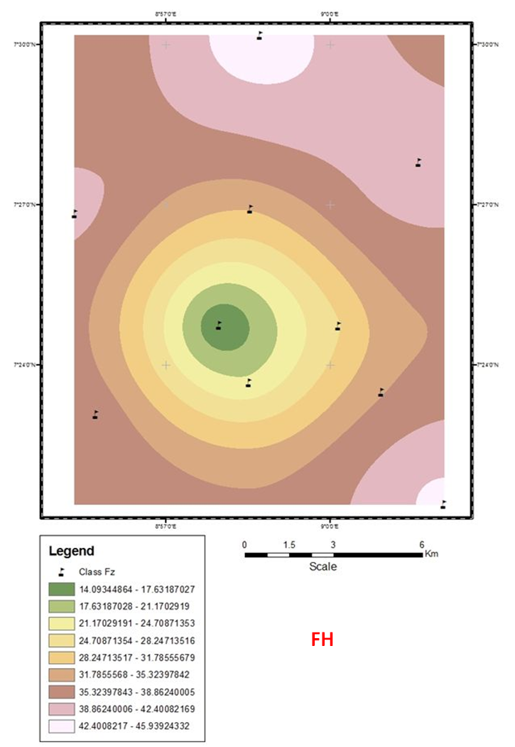
- The spatial autocorrelation of plume dispersion is applied in this research to interpolate the gathered data and establish the values from point to point within the study area, resulting in variograms (Appendix 3). The variograms model the difference between the value of plume concentration at each intervalled kilometer (1 – 10), according to the distance and direction between them. As a key function in geostatistics, it is used to fit a model of the spatial correlation of the plume concentration data for this study. Therefore, the variograms also represents both structural and random aspects of the dispersion coefficients of plume within a known distance of 10 km intervalling at single km. As shown on the variograms (Appendix 3), values increase with increasing distance of separation until it reaches the maximum (C) at a distance known as the “range” (a). If at a distance nearly equal to zero, (h 0), the variogram value is greater than zero, this value is known as the “nugget-effect” (C0). The total-sill of the variogram (S) is C+C0. Often C is also treated equal to the sill of the variogram model fitted to the experimental variograms and the nugget effect (C0). Both C0 and the sill (S) characterize the random aspect of the data, whereas the range (a) and C characterize the structural aspect of the deposit of plume. The analysis is consistent with [31] and [32].The application of this model to this study has aided the establishment of the predictability of values at those locations across a relatively wider area affected by plume, yet not sampled by this study. Also, the technique reveals the dispersion pattern of plume under the various atmospheric stability classes (defined by prevalence of weather conditions and time of day), as well as on the basis of vertical and horizontal orientations. The weights are optimized using the variogram model (generated and shown as Appendix 3), the location of the samples and all the relevant inter-relationships between known (and even unknown) values for specified (and even unspecified) locations within the study area. A "standard error" function is also provided within the variogram which allows for the quantification of confidence levels for all locations analysed.Generally, for both vertical and horizontal dispersion coefficients in all atmospheric stability classes, the rate of plume dispersion is shown to be outwardly increasing, while the direction of plume travel is determined by the prevailing condition of winds at any given time. Thus, the output variograms for plume deposition at the study area exhibit an omni-directional (as against directional) orientation, and are sufficient for kriging data even as spatially irregular as the results of the plume dispersion coefficients appear. Finally, the distribution of plume on the variograms seems spatially correlated in a radial, omni-directional orientation.
4. Discussion
- The environmental consequences of cement production at the study area are glaring even to a passive observer. Soil and plant texture is observed to be affected by fugitive dust and plume deposits over the years. With the installation of taller stacks (75m as against the previous 55m stacks), the effective stack height is increased at which point the plume exits at a higher buoyancy level and travels farther down wind (depending on the prevailing weather conditions) therefore, deposition occurring further away from the source of emission.Furthermore, plume dispersion exhibits a seasonal pattern of variation where plume deposition is denser during the rainy season when the wind conditions are relatively stable, and more scattered during the dry windy season.Although daily averages of plume dispersion vary across the atmospheric stability classes as well as along their vertical and horizontal orientations (Table 5), they are found generally occurring higher and denser away from the factory. Since plume, fugitive and cement dust contains heavy metals and pollutants hazardous to the biotic environment, with adverse impact for vegetation, human and animal health and ecosystems [33, 34], the rate of concentration observed is considered unhealthy for the biotic environment.
5. Conclusions
- Summary of the major findings indicate that: the highest plume dispersion coefficient values are recorded for the ‘unstable’ climatic stability class ‘A’ with least values recorded for the relatively ‘stable’ stability class ‘F’; the plume dispersion coefficients for the study area are estimated to be generally high; the ANOVA result of plume dispersion coefficients is found to be significant, implying that the values of the means differ more than would be expected by chance alone; the variograms show that plume deposition amounts increase with distance away from the emission source (the stacks at the cement factory), and is radially omni-directional in orientation. The implication is that the observed daily average values of both PM10 and PM2.5 are higher than the WHO [35] permissible limits for all stability classes except for DH, EH and FH stability/orientation categories. This result spells adverse effect for both human, animal and plant population within the 10-kilometre study radius.It is therefore, recommended that:● Deliberate reforestation efforts using species with high pollution tolerance index such as Azadirachta indica, Albizzia lebbek, Aegle marmelos, Annona squamosa, Bambusa bambos, Butea frondosa, Cassia fistula, Cordia myxa, Delonix regia, Ficus religiosa, etc.;● Consistent and periodic inquiry into the environmental status of the area is suggested to ensure sustainability in the face of cement production at the factory;● Selective Catalytic Reduction (SCR) and Selective Non-Catalytic Reduction (SNCR) systems should be adopted at the factory kilns to reduce drastically, the amount of plume emissions during production; and,● Human, animal and agricultural populations should only be located either within the first 2 - 3 km or from 11 km away from the factory (avoiding km 4-10 which are areas of high plume deposition levels) to reduce the risk of exposure to plume from the factory.
ACKNOWLEDGEMENTS
- The author is grateful to the community members of Tse-Kucha and Tse-Amua for their cooperation throughout the period of this research. Mr. Iortyer Gyenkwe and Mr. Solomon Ukor were also helpful during field work.
Appendix 1
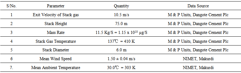 | Field Survey Data for Plume Modelling |
Appendix 2
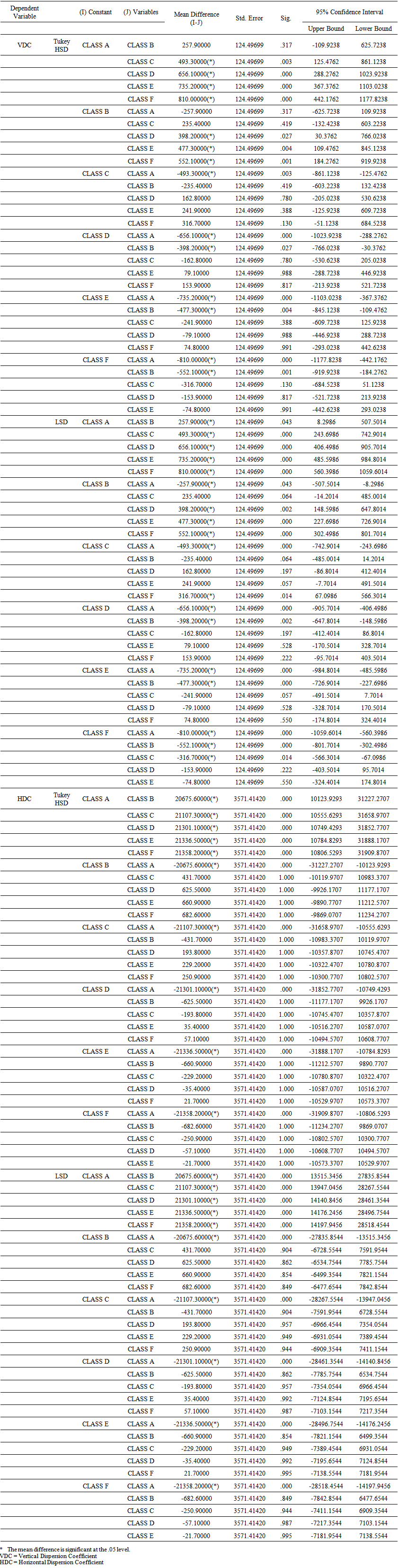 | Post Hoc Multiple Comparisons of Atmospheric Stability Classes |
Appendix 3
- Variograms showing plume distribution in x and y orientations for all stability classes.
 | Figure 4(a). Variograms showing plume distribution in x and y orientations for all stability classes |
 | Figure 4(b). Variograms showing plume distribution in x and y orientations for all stability classes |
 | Figure 4(c). Variograms showing plume distribution in x and y orientations for all stability classes |
 | Figure 4(d). Variograms showing plume distribution in x and y orientations for all stability classes |
 | Figure 4(e). Variograms showing plume distribution in x and y orientations for all stability classes |
 | Figure 4(f). Variograms showing plume distribution in x and y orientations for all stability classes |
 | Figure 4(g). Variograms showing plume distribution in x and y orientations for all stability classes |
 | Figure 4(h). Variograms showing plume distribution in x and y orientations for all stability classes |
 | Figure 4(i). Variograms showing plume distribution in x and y orientations for all stability classes |
 | Figure 4(j). Variograms showing plume distribution in x and y orientations for all stability classes |
 | Figure 4(k). Variograms showing plume distribution in x and y orientations for all stability classes |
 | Figure 4(l). Variograms showing plume distribution in x and y orientations for all stability classes |