1. Introduction

Sustainability is taken to mean that all resources are used efficiently both within and between generations and that the productive base of society is more or less preserved overtime[1]. In Tanzania watershed resources are found to support directly welfare of most households in the area and or adjacent by means of food, construction materials, medicines, firewood, charcoal and water[2]. The watershed also supports households’ wealth in the form of asset such as livestock. Given the higher value to and the dependence of local communities on the watershed resources, it means that conservation of watershed resources requires additional policies to prevent an increase of poverty in the country. Thus the implementation of the integrated watershed management is paramount.

The concept of the integrated watershed management emerged in the 1970’s following the warning of the scientific community on the state of the environment on the earth. As one of the first events that emphasized the environment management in the framework of development, the UN Conference on Human Environment of 1972 can be mentioned. The conference urged the governments to pay attention on conservation of natural resources while pursuing their development goals. However, the implementation of conservation and development issues remained as a separate goal for a long time by many governments. The Brundtland report defines sustainable development as the development that meets the needs of the current generation without compromising the ability of the future generation to meet their needs. The report marked the start of the integration of both the development goals and the conservation goals in the planning.

In 1992, at the occasion of the Rio conference of the WCED, the Agenda 21 was formulated. The key message of the Agenda was the establishment of a framework for the integrated watershed management. The Agenda also included guidelines for the promotion of alternative income generating activities. The Agenda 21 played an important role for the integration of conservation and development goals. It was indeed the first time that the views of economists and social scientist were incorporated in watershed management[3]. Today, it is considered a basic human responsibility to ensure that both natural and human systems are sustained in healthy condition for the sake of the earth and people. Vishnudas et al[4] point out that, for the watershed to be sustainable, land, forest and agriculture must be sustainable first. However, the bench mark or indicators to guide of the status of the sustainable development of which both the natural resources and welfare of the people who are depending of these resources is lacking. The rest of the paper is organized in four sections. After introduction, the second part presents materials and methods, the third section details empirical literature on the technical efficiency and sustainability indicators. Section four presents the theoretical framework followed by the methodology. The stochastic frontier methods are discussed. This is followed by the discussion of the study results in section five. Lastly are the concluding remarks and policy implications in section six.

2. Materials and Methods

2.1. Location and Physical Characteristics of the Study Area

The area for this study is the Sigi catchment, with a total area of 1100 km². It is located between latitude 4^o 80' and 5^o 26' S and longitude 38^o 58' and 39^o 10' E in Tanga region, the North Eastern part of Tanzania (Figure 1). The basin is situated on the eastern slopes of the of the East Usambara mountain block of the Eastern Arc Mountain forests, at altitudes between 2 and 1200m above mean sea level. The basin comprises most of the forests of the East Usambara Mountain. These forests occupy most of the upstream of the basin.

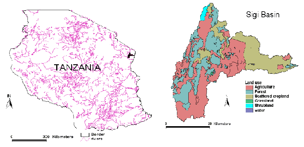Figure 1. Location of the study area in Tanzania

Figure 2. Sigi catchment, topography, river networks and stations

The watershed is formed by the permanent and seasonal rivers. Many rivers are small and highly dependent on rainfall variability. The permanent rivers include Kihuhwi, Semdoe, Muze and the Sigi River (Figure 2). All rivers flow from different sources and joins to form the main Sigi River. The Sigi River flows throughout the year to the Indian Ocean. The average monthly flow peaks occur in the period of April – June and in October – December and the annual average flow is 431mm.

2.2. Rainfall and Temperature

The area has a bi – modal rainfall pattern with two rain seasons. The long rain period is March – May and the short rain period is October – December. For the period between 1995 and 2005, the monthly average rainfall stood between 30 and 174 mm (Figure 3). On the other hand, the maximum temperature ranges between 28℃ and 35℃ and the minimum temperature between 17℃ and 23℃ (Figure 4).

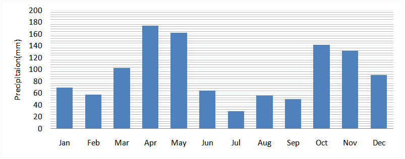Figure 3. Rainfall distribution for 1995 – 2005 at Lanzoni weather station

Figure 4. Temperature distribution 1995 – 2005

3. Relevant Literature on Technical Efficiency and Sustainability Indicators

An indicator is something that helps to understand the past, present and future state of resource in question. Identifying and developing environmental sustainability indicators have been recognized as the cornerstone of the UN-World Water Assessment Programme. The early efforts of UNESCO’s International Hydrological Decade, subsequent International Hydrology Programme (IHP) phases, FAO, IAEA and UNEP as well as professional organizations have produced several important methodological guidelines toward indicator development. It is argued that, most indicator initiatives aimed at providing information at a national level for state-of-the-environment reporting[5, 6, 7, 8] or for answering specific policy questions at national and international levels[9, 10, 11]. Environmental sustainability is a relatively new phenomenon in comparison to indicators of economic and social aspects[12]. The central idea with the environmental sustainability indicators is to ensure meeting the current human needs without undermining the capacity of the environment to provide for those needs over the long term[13].

The current water resources sustainability indicators include the water poverty index (WPI) by Sullivan[14], the Canadian Water Sustainability Index (CWSI) by Policy Research Initiative[15] and the Watershed Sustainability Index (WSI) by Chaves and Alipaz[16]. WSI based on UNESCO framework called HELP (Hydrology, Environment, Life and Policy). WSI is a watershed specific index that takes into account cause-effect relationships and considers policy responses implemented in a given period as part of the basin’s sustainability. The WSI includes the extent of forest cover in the watershed. Policy Research Initiative[15] states that, the catchment is sustainable when are covered by about 40% of natural vegetation. A catchment is also said to be sustainable if there is 20% or greater improvement in catchment conservation.

The efficiency in production has been examined for more than 60 years[16, 17]. The technical efficiency (TE) is defined as the ratio of the firm or the farmer actual production to the optimal output. The TE reflects the ability of the producer to obtain maximum outputs from a given set of inputs. Therefore, the producer is said to be technically efficient when the actual output is equal to the optimal output and the same producer is said to be inefficient when the actual production is less than optimal output or the frontier output[17]. For the given production processes, technical efficiency would be measured theoretically within the range . The literature proposes two alternative approaches for the estimation of TE. The first approach is the SFA, the parametric Stochastic Frontier Analysis[18, 19, 20, 21, 22, 23]). The second approach is DEA, the non-parametric Data Envelopment Analysis[24].

It is concluded from the literature that sustainability of water resources can be effectively achieved as the poverty within the community decreases. Natural assets such as land, forests and water have linkage between watershed management and livelihood, thus, watershed management that focuses on natural resources alone has a limited impact on livelihood and poverty[2]. This conclusion however does not put out clear that the established relationships are location specific and cannot be used to generalize the situation in other areas. This therefore calls for a site specific study to reveal the actual condition of the natural environment and livelihoods issues in order to ascertain the clear link between watershed resources and the welfare condition of the local community.

4. Analytical Framework

In this paper, effort was made to develop addition indicator variables that are important in the addressing the sustainable watershed management. The indicators are both socioeconomic and environmental based attributes. The livelihood - welfare based indicator proposed is the technical efficiency (TE) indicator. TE indicator is considered as single representation of the welfare, livelihood and watershed health status. It is made from the idea embodied in crop production – which is the main livelihood of the people in the study area. We adopt the sustainable livelihood framework[25, 26] in understanding the importance of watershed resources and transformation structures in realizing welfare goals. The sustainable livelihood framework is one of the most common diagnostic tools employed in development and interventions. The framework explains how complex issues of rural development could be approached and successfully addressed[25, 26]. The sustainable livelihoods adopted from[25, 26] is a framework showing the relationship among the context of the farmers’ assets, transformation structures, livelihood strategies, and livelihood outcomes. The framework shows the indirect relationship between livelihood outcomes and households’ assets and the role of transformation structures and the watershed resource harvesting strategies. In this paper effort has been to downscale the analysis to have indicators at small unit (the watershed) and link the resource utilization and the welfare of the local communities around watershed resources. We believe that to achieve environmental resource sustainability requires carefully balancing human development activities and the resources upon which activities are done on[3, 27].

4.1. The Model Specification

The TE is determined based on the stochastic frontier analysis (SFA). This method is chosen based on its ability to distinguish the error term between the two error sources: the random error term that represents the inefficiency component and the effects of factors beyond the control of the farmer and the random error term that represents the inefficiency due to farm and farmer specific attributes[21, 26]. The specification of the model follows the procedure by[28] and incorporates two parts. In the first part the efficient production frontier is estimated as a function of control variables and specified as indicated below:

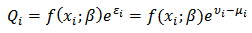(1)

Where is production of the i-th observation (farm); is a vector of explanatory variables related to production inputs and other control variables of the i^th observation; is a parameter vector and is the error term represented by the terms and .

● The term is for the random variations in production due to observation and data measurement errors, uncontrolled factors etc. is assumed as identically and independently normally distributed: .

● The term is a random non-negative variable, which is associated with the measure of technical inefficiency relative to the stochastic frontier. is assumed to be truncated normally distributed.

In the second part, the stochastic frontier estimation involves the estimation of the function that relates the inefficiency measurement obtained in the first stage with a set of explanatory variables corresponding to farm and farmer specific characteristics. The inefficiency function takes the form:

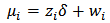(2)

Where is a vector of variables representing the technical inefficiency of the i^th observation; corresponds to a parameters vector and represents the error term.

Finally, we combine equation 1 and 2 and define TE as the ratio of the observed output, and the maximum feasible output . This ratio is representing the technical efficiency for the i^th observation:

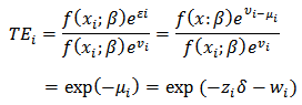(3)

4.2. The Empirical Model

The empirical model to estimate the TE can take either the Cobb-Douglas production function (CDPF)[29] or the translog production function (TLPF)[30]. The TLPF formulation assumes the existence of a non linear relationship between the output and the inputs. In addition, the production elasticities are not constant. Because of this flexibility most TE studies have used this specification[22, 23, 31, 32]. In the study area, the TLPF specification is adopted and the specification of the model for the assessment of the TE of farmers is made based on three factor inputs, as specified in Equation 4[22].

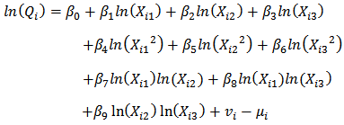(4)

Where represents the value of harvest (kg); represents the j^th input of the i^th farm household ; is the total area planted (in acres) (FS); represents family labour (number of adults) (FL) and represent the expenditure on hired labour (Tshs) (CP); are coefficients to be estimated and represent the random error and is the error term that reflects the technical inefficiency. The inefficiency model is estimated based on ten variables that reflect the technical inefficiency measures, as specified in Equation 5.

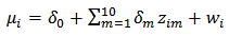(5)

where represents the crop yield potential (CY); represents the quantity of firewood collected by household per year (FW); is the household size (HS); represents the age of the head of the household (AG); represent the male gender of the head of the household (MA); represents access to credit by the household (CR); is the education level of the head of the household (ED); represents the receipts of remittances by the household (RE); represents the migration status of the head of the households (MI); represents the average income of the household (HI); are coefficients to be estimated and is the error term that follows the truncated normal distribution.

The parameters of the production frontier function defined by equation (4) and the inefficiency model defined by equation (5) are jointly estimated by the Maximum Likelihood (ML) method, using FRONTIER 4.1[33]. The ML estimation provides the consistent estimators for variance parameters given by

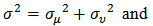(6)

(7)

Where the parameter refers to the proportion of total variance that is explained by the variance of the inefficiencies and whose values are between 0 and 1. Corresponds to the variance of the stochastic model and corresponds to the variance of the inefficiency model. is the total variance.

The performance of the FRONTIER 4.1 model for estimating the parameters of technical efficiency is assessed through testing hypotheses[18, 19, 20, 21, 22, 23]. These hypotheses are made to guide the assessment of the model performance by considering two issues: the first one is the adequateness of the functional form of the model. To test for the adequateness of the functional form of the model for the joint estimation (Equation 4 and 5), the procedure is to evaluate the significance of the coefficients of the parameters estimated. To achieve this we test the hypothesis (Equation 8).

(8)

The relevant test is the generalized likelihood-ratio (LR) test statistic. This statistic is obtained by estimating the above joint model in two ways; first we restrict the model to include only 3 inputs of production. From the restricted model we obtain the likelihood value and secondly we estimate the unrestricted model and we obtain the likelihood function value We use these two values and to define the test statistic in the Equation 9[22].

(9)

The test statistic has a distribution or a mixed distribution with degrees of freedom equal to the difference between the number of the estimated parameter in the restricted and the unrestricted model. The second issue is the significance of the inefficiency model specified and the inefficiency variables. To evaluate the significance of the inefficiency model, the relevant hypothesis tested is one on whether the model is stochastic or not. The inefficiency model is valid when it is stochastic. This is evaluated by testing the hypothesis that the variance due to the inefficiency model (Equation 10) is not present i.e.

(10)

The decision to reject or not is reached by the estimated value of in the joint model. The mixed chi square test is used. The relevant decision is reached by assessing the significance of the statistics established by considering the likelihood function value of model with inefficiency (unrestricted) and without inefficiency variables (restricted). The hypothesis is rejected if the is greater than the standard value obtained from the mixed chi square distribution table[33]. This also involves assessment of the significance of the individual coefficients from the estimated model and the t-ratio.

5. Data and Descriptive Statistics

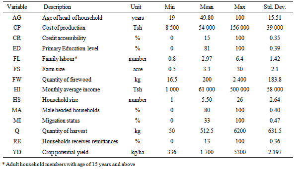
Direct observations, group discussions and semi structured questionnaires were the main data collection approaches employed in 27 villages within the Sigi basin in 2008/9. Individual household interviews were conducted on 764 smallholder farmers’ households across the 12 sites as delineated in the SWAT model set for the Sigi Basin[34]. The SWAT model provided the crop yield potential for each site within the basin. The crop yield was validated by the household level data on crop production. The summary of the descriptive statistics of the variables used to establish the technical efficiency in crop production is presented in Table 1. The average maize harvest per household was 513 kg, with the minimum and maximum of 50 and 6 200kg. The larger amounts of harvest correspond to the relatively large farm sizes and higher crop yield potential. On average the household size was five members and the average adult members who supply family labour was three members. The education level of the heads of the household shows that majority (80%) only have a primary level of education. The average household income per month was TSH 60 000 or USD 50. This indicated a prevalence of poverty for the majority of the household members in the study area. Only 15% of the households have accessed credit and the main source of credit was from the SACCOS, the Savings and Credit Cooperatives Societies. In terms of remittances, 13% of sampled households indicated to receive cash income in the form of remittances from relatives outside the study area. Assessment of the migration pattern of household members indicated that about 33% of respondents were migrants who came during 1970’s and 1980’s primarily for the search of farm land and also employment in sisal and tea estates. The average quantity of firewood collected per year per household was 0.2 ton and the maximum amounts to 2.4 ton per household per year. The lack of an alternative source of energy, such as electricity, in the study area was the main factor for the higher quantity of firewood use by households for cooking and lighting.

Table 1. Summary of descriptive statistics of the key variables used in the analyses

5.1. Model Performance Results

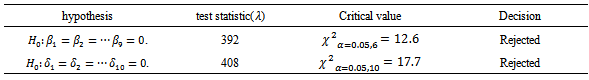
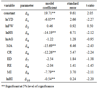
We evaluate the performance of the estimated TLPF by testing the hypotheses on the overall significance of the model and the estimated parameters (Equation 8 and 10). The hypothesis expressed by Equation 8 was rejected at 5% level of significance (Table 2). This implies that the specified TLPF fits the data well. The hypothesis of Equation 10 was rejected (Table 2).

This implies that the deviation of the actual output by the farmers in the study area was both due to data noise and too technical inefficient. This is also supported by the estimated (significant) coefficients of the individual inefficiency variables (Equation 5), whose results are presented in Table 4.

Table 2. Test of hypotheses for the stochastic production frontier and inefficiency model

5.2. The Technical Efficiency Results

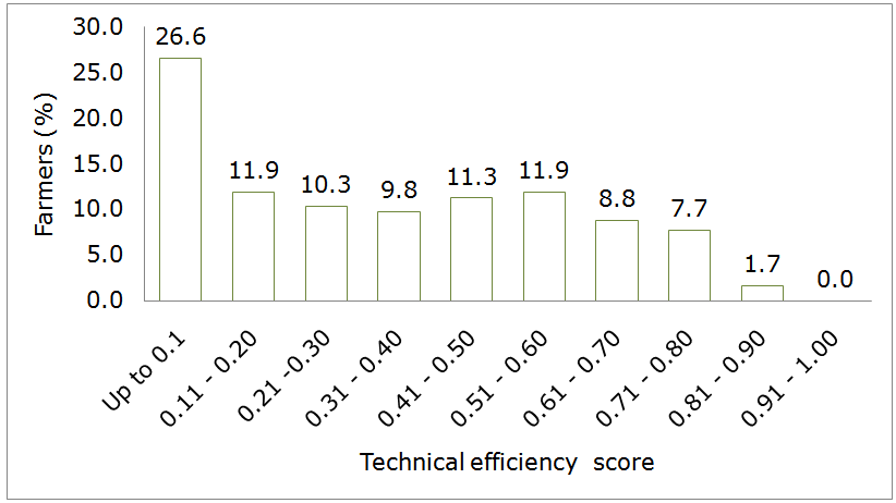Figure 5. Distribution of the technical efficiency

The estimated mean technical efficiency of maize is 33% (Table 3 and Figure 5) implying that there was substantial technical inefficiency in maize farming. On average, smallholder maize farmers in the study area incur about 67% loss in output due to technical inefficiency.

Table 3. Variance parameters

On Figure 5 it can be seen that the majority of the farmers had a TE below 0.3; none of them had TE of 0.9 and above. This explains why farmers in the study area were constantly looking for more crop land and thus causing forest loss due to clearing to establish new farms. The key message from this result is that deliberate efforts are required for improving the TE. If causes of inefficiency in crop production are addressed, this could save a significant amount of forest.

The analysis of the TE scores indicates a significant difference between the upstream and the downstream part of the watershed. On average, the TE score of the upstream farmers found to be 0.4 while the TE score is 0.2 for the farmers in the downstream part. The Mann-Whitney U test was performed to establish any significance differences of the TE between the upstream and downstream farmers. The null hypothesis of no significance difference was rejected with Z=-8.7 at 5% level of significance. The upstream had an average rank of 430.12 while the downstream had an average rank of 279.17. This implies that the upstream part of the watershed has more productive land than in the downstream part. Thus the upstream part attracted many households to establish their farms. If this is left to continue it is going to cause further degradation of the watershed due to agricultural expansion.

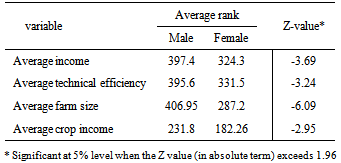
5.3. Factors Influencing the Technical Efficiency

Table 4. Factors influencing technical inefficiency in the study area (inefficiency model)

The identified factors influencing the technical efficiency in the study are presented in Table 4. These are the key variables to look at when addressing the sustainability of watershed resources in the study area. There was clearly considerable scope for the technical efficiency increase and therefore the sustainability of watershed resources in the study area. The significant negative relationship between the inefficiency and most the variables is an indication of the opportunity to increase the technical efficient in the study area.

The variable crop yield had a positive and statistically significant relationship with the technical efficiency as expected. This implies that farmers who cultivates in areas with high crop yield would have high the technical efficiency. High yield areas enable farmers to maximize output per unit area of cultivated land at the low costs. In the study area, farm expansion by households was made by converting forests to agricultural land and these areas had a higher yield potential than the land that was under continuous cropping. Credit availability and the household income variables had positive and significant influences on the technical efficiency. The technical efficiency would be high for households with access to the credit facilities and when the average income increases. This implies that income enhancing efforts such as credit to farmers could be an opportunity to increase technical efficiency in crop production and therefore the sustainability of the watershed. The enhanced income and credit opportunities could enable farmers to purchase the inputs such as fertilizers and improved seeds, to have the storage and be able to transport the crops to the markets for higher prices than waiting for buyers who buy at the farm gate prices which are extremely low.

The increase of household members was found to influence positively the technical efficiency as expected. This means that a large number of adult members of the households ensure abundant household labour supply. In the study area crop production was highly labour intensive. The more the adult members of the households the more labour for crop production and thus the high the technical efficiency.

Table 5. TE, farm size and crop income differences for the male and female headed households

Households headed by the male members were found to have relatively higher technical efficiency than households headed by female members. The low TE by female headed households was contributed by the low income for the female headed households. In literature female headed households in Sub Saharan Africa (SSA) are found to have relatively lower average income than the male headed households[34, 35]. The low income prohibits the female headed households to use the agricultural inputs such as hired labour and inorganic fertilizers important for raising the crop productivity. In the study area the average income of the female headed households is statistically significant lower than the income of the male headed households. The Mann Whitney U test leads to the rejection of the null hypotheses of no differences in income, TE, farm size and crop income at 5% level of significance between male and female headed households in the study area (Table 5).

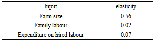
5.4. Elasticity of the Technical Efficiency

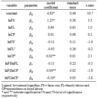
The estimated coefficients in the TLPF (Table 6) do not have a straightforward interpretation. It was necessary to estimate the output elasticity for each of the inputs used in order to have a meaningful interpretation[21, 36]. Equation 11, 12 and 13 below are used to estimate the elasticity of the output with respect to the farm size (FS), family labour (FL) and the expenditure on hired labour (CP). In these equations, coefficients and mean values of the respective inputs are used to estimate the elasticity.

Table 6. Final MLE estimates for the efficiency model

Upon utilization of the mean values (Table 1) and the estimated coefficients (Table 6) in equation 11, 12 and 13 the elasticity for the inputs in the TLPF is estimated (Table 7).

(11)

(12)

(13)

The estimated elasticity for all inputs (Table 7) is positive and they suggest that the TLPF is well behaved in representing the production technology in the study area. From these results it can be concluded that the increase of the inputs by 1% would result to an increase of output by less than. This indicates that that the production in the study area was operating at decreasing return to scale. That is additional application of the current inputs would, in relative terms, result in a smaller increase in crop output. This suggests that, to improve crop production, there is a need of introducing other inputs in addition to those that are currently used.

Table 7. Elasticity of the farm size, family labour and cost of hired labour

6. Conclusions

The technical efficiency indicates that the crop productivity in the study area is low. Farmers do not have means of investing on land in order to improve crop production. This has resulted to the majority of the farmers to rely on additional land for cultivation in order to compensate for the declined crop harvest through farming on forested areas considered to be rich in natural crop yields. The production in the study area is operating at decreasing return to scale. This implies that additional application of the current inputs would, in relative terms; result in a smaller increase in crop output. This suggests that, to improve crop production, there is a need of introducing other inputs in addition to those that are currently used. The income from crops is found to influence positively the welfare of households in the area. This implies that watershed resources have a greater role to play on the welfare of the communities because of the direct relationship between crop cultivation and the watershed environment. Therefore there is a need to take into account the sustainability of the watershed resources when setting development policy in the study area. The higher technical efficiency in crop production would enable households to harvest large quantity of crop output per unit area. This could limit the proportion of the agricultural land in the catchment. The cause of the inefficiency is therefore needed to be addressed in order to have sustainable watershed resources and the improved human welfare.