Shadia A. H. Fathy 1, Fatma F. Abdel Hamid 1, Mohamed A. Shreadah 2, Laila A. Mohamed 2, Mohamed G. El-Gazar 2
1Biochemistry Department, Faculty of Science, Ain Shams University, Cairo, Egypt
2The National Institute of Oceanography and Fisheries, Kayet Bay, Alexandria, Egypt
Correspondence to: Laila A. Mohamed , The National Institute of Oceanography and Fisheries, Kayet Bay, Alexandria, Egypt.
| Email: |  |
Copyright © 2012 Scientific & Academic Publishing. All Rights Reserved.
Abstract
This paper presents water quality analysis of three sites located in the coastal area of Alexandria, Egypt. Principal component analysis (PCA) approach was used to develop water quality index (WQI). PCA results revealed that Nubaria and Umoum drains were the most highly polluted sampling sites and supposed to be hotspots of environmental pollutants due to industrial, agricultural and domestic wastes disposed and eluted compared to Kilo 21 drain which could be considered the control site for the present study. The findings with the help of principal components suggested are being of great importance in establishing guidelines for the administration of water sources and the improvement of water quality in these areas.
Keywords:
Water Quality, Principle Component Analysis, Physicochemical, Environmental Pollutants
Cite this paper:
Shadia A. H. Fathy , Fatma F. Abdel Hamid , Mohamed A. Shreadah , Laila A. Mohamed , Mohamed G. El-Gazar , "Application of Principal Component Analysis for Developing Water Quality Index for Selected Coastal Areas of Alexandria Egypt", Resources and Environment, Vol. 2 No. 6, 2012, pp. 297-305. doi: 10.5923/j.re.20120206.08.
1. Introduction
The quality of water is a very sensitive issue and it is identified in terms of its physicochemical parameters[1]. The particular problem in the case of water quality monitoring is the complexity associated with analyzing the large number of measured variables[2]. The data sets contain rich information about the behavior of the water resources. Multivariate statistical approaches allow deriving hidden information from the data set about the possible influences of the environment on water quality[3].Principal component analysis (PCA) is the method that provides a unique solution, so that the original data can be reconstructed from the results. Principal components (PCs) actually take the cloud of data points and rotate it such a way that maximum variability is visible. In other words, it identifies the most important gradients. In recent years many studies have been done using PCA in the interpretation of water quality parameters, Lohani and Todino[4] utilized principal components technique to provide a quick analyticalmethod for the water quality of Chao Phraya River in Thailand. Shihab,[5] also used this technique in order to describe the variation in water quality in Saddam dam reservoir. Principal component analysis has been successfully applied to sort out hydrogeological and hydrogeochemical processes from commonly collected ground water quality data[6] and[7]. To establish the spatial and temporal variations in water quality, regular monitoring programs are required, thus PCAis being used in this study.The PCA methods contained in the statistical SPSS program was applied to the chemical concentration data in order to study the physicochemical variables, heavy metals and some organic pollutants capable of promoting a characterization of the hydrochemistry of the region and to identify the fundamental factors that govern the general behaviour of the polluted water sources.
2. Materials and Methods
Water samples collected from study areas were analysed for their physicochemical parameters, also concentrations of some heavy metals and organic pollutants were determined. Data submitted from PCA were used for calculating the water quality index for each area.
2.1. Study Areas
Water samples were collected 1m depth (approximately the mid-depth of thewater body of uniform temperature[8])from three sites along the Mediterranean coast of Alexandria, Egypt (Figure 1); Kilo 21 (31⁰ 05' N - 29⁰ 53' E),Nubaria (31⁰ 07' N-29⁰ 53' E) and Umoum (31⁰ 07' N-29⁰ 53' E) during winter and summer of the year 2011.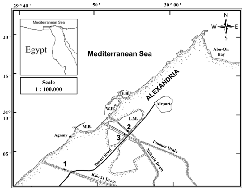 | Figure (1). A Map showing locations of the sampling sites; 1- Kilo 21 (Control site), 2- Nubaria (Site I) and 3- Umoum (Site II) drains. (M.B.: El-Max bay; W.H.:Western harbor; E.H.: Eastern harbor; L.M.: Lake Mariut) |
2.2. Physico-chemical Properties of the Water Samples
Surface water samples were collected during summer and winter in triplicates from each site with clean plastic buckets. Preservation and transportation of the water samples to the laboratory were as per standard methods provided by the Canadian Council of Ministers of the Environment[8]. Water temperature was measured on the site using mercury thermometer. pH was measured using digital pH meter (Model 201, Orion Research INC.). Total alkalinity was determined by the titration using 0.01N hydrochloric acid and methyl orange as indicator according to standard methods[9]. Density and transparency of water was measured according to the American Public Health Association (APHA) [10]. Turbidity was measured by Nephelometer using 0.02 NTU standards[11]. Salinity, electric conductivity (EC) and total dissolved solids (TDS)were measured using Salinometer (Thermo Electron Corporation, model: Orion 150A+, USA). Chlorinity was estimated by Mohr-Knudsen titration[12]. Dissolved oxygen was fixed immediately after collection and then determined by Winkler’s method[13]. Samples for biochemical oxygen demand (BOD5) were incubated in laboratory for five days at 20 0C[14]. Chemical oxygen demand (COD) and total nitrogen (TN) were estimated according to APHA[8]. The method used for the determination of oxidizable organic matter (OOM) was that described by Food and Agriculture Organization (FAO)[15], while total phosphorus (TP) was analyzed according to standard method of Unites States Food Protection Agency (USEPA)[16]. The average, maximum and minimum values for each season have been considered. The present study reports the seasonal pattern of the physicochemical parameters at these three sites.
2.3. Determination of the Heavy Metals
Water samples were digested according to the method described in APHA[10]. The levels of iron (Fe), copper (Cu), zinc (Zn), lead (Pb), cadmium (Cd) and mercury (Hg) in digests of water were determined using atomic absorption spectrophotometer (Shimadzu AA-6800, Japan) equipped with different cathode lamps with air acetylene flame atomic absorption (FAA) technology (Thermal atomization) for Cd, Pb, Cu, Fe, Zn, while atomic absorption cold vapor technique was used for Hg. The cathode lamps had wave length range from 190 to 900 nm. The absorptionwavelengths used for measurements and detection limits are listed in Table (1). All reagents used were of analytical grade were used for sample digestion and preparation of the standards. The digestion and analytical procedures were checked by analysis of standard reference materials (ORMS-2). A replicate analysis of these reference materials showed a good accuracy, with recovery rates for metals between 94% and 102%. To prevent contamination, all materials associated with trace metal sampling and analyses were thoroughly acid cleaned before use. Glassware and Teflon® vessels were treated in a solution 10% v/v nitric acid for 24 h and then washed with distilled and deionized water.| Table (1). The absorption wavelengths and detection limits of the metals under investigation |
| | Metal | Symbol | Absorption wavelength | Detection limit | | (nm) | (ppt) | | Iron | Fe | 248.3 | 0.04 | | Copper | Cu | 324.8 | 0.03 | | Zinc | Zn | 213.9 | 0.07 | | Lead | Pb | 217.0 | 0.08 | | Cadmium | Cd | 228.8 | 0.01 | | Mercury | Hg | 253.7 | 0.005 |
|
|
2.4. Determination of Organic Pollutants
One liter of water was poured into glass separator funnel, extracted twice with 40 ml of methylene chloride. The extract was stored in dark at low temperature (~5℃). Before analysis, the stored extracts were evaporated to dryness in a rotary evaporator at 30℃ under reduced pressure. The residue was re-dissolved in 1ml of n-hexane before fractionation with column chromatography[17]. The extracted solvents were concentrated with a rotary evaporator down to 2 ml (maximum temperature: 35℃), followed by concentration with a pure nitrogen gas stream down to a volume of 2 ml (one milliliter was cleaned-up with column chromatography for Polycyclic Aromatic Hydrocarbons (PAHs) and the other one for Organochlorine pesticides (OCPs) and Polychlorinated Biphenyls (PCBs). For determination of PAHs, The first milliliter of the extracted volume was measured for total hydrocarbons using fluorimete then was passed through the silica column prepared by slurry packing 10 g of silica, followed by 10 g of alumina and finally 1 g of anhydrous sodium sulfate. Elution was performed using 40 ml of hexane (aliphatic fractions), then 40 ml of hexane/dichloromethane (9:1), followed by 20 ml of hexane/dichloromethane (1:1) (which combined contain PAHs). Copper powder was added to the obtained fractions and the change of the copper color from brassy red into black was taken as an indication of sulfur removal that interfere in GC-MS (Gas Chromatograph-MassSpectrometer) analysis[18], while the second milliliter was used for determination of OCPs and PCBs, where it was passed throughflorisil column prepared by slurry packing 20 g of florisil, followed by 10 g of alumina and finally 1 g of anhydrous sodium sulfate. Elution was performed using a 50-ml mixture containing 70% hexane and 30% dichloromethane for pesticide fractions. copper powder was was added to the obtained fractions and the change of the copper color from brassy red into black was taken as an indication of sulphur removal that interfere in GC-MS analysis[18]. Finally, eluted samples were concentrated under a gentle stream of purified nitrogen to about 0.3 ml, prior to injection into GC-MS; Trace-Ultra coupled to DSQ- II MS (thermo electron S.P.A) equipped with splitless injector and a fused silica capillary column; Thermo TR-35 MS (30m, 0.25mm and 0.25μm) with 35% phenyl polyphenylene-siloxane.
2.5. Water Quality Index (WQI)
Principal component analysis (PCA) is applied for multivariate data derived from the different variable analysis of water from sampling sites. PCA was carried out using statistical package for the social sciences- version 18 (SPSS-18). The data contain 33 variables: All physicochemical parameters, heavy metals, THCs, PAHs, OCPs and PCBs. Data submitted for the analysis were arranged in matrix, where each column corresponds to one variable component and each row represents a sampling site. The number of factors extracted from the variables was determined according to Kaiser’s rule. This criterion retains only factors with Eigen values that exceed one. The first step in the multivariate statistical analysis was application of PCA with the aim to group the individual parameter components by the loading plots for the investigated contaminated sites. The use of PCA to water quality assessment has increased in recent years, mainly due to the need to obtain appreciable data reduction for analysis and decision[19]. Water quality index (WQI) is calculated according to the following formula: 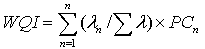 For PC Assessment model where n: The number of effective components, λn, are the Eigen values of the effective components, Σ λ is sum of the Eigen values and PCn are the n critical principal component factor scores[20].
3. Results and Discussion
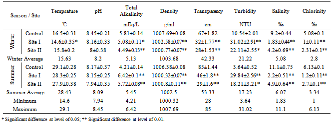
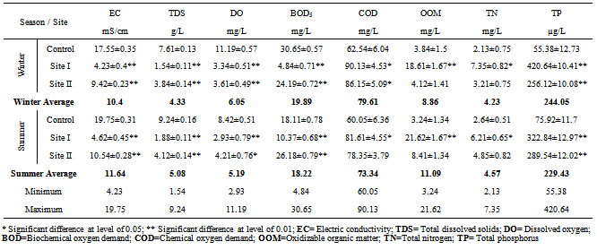
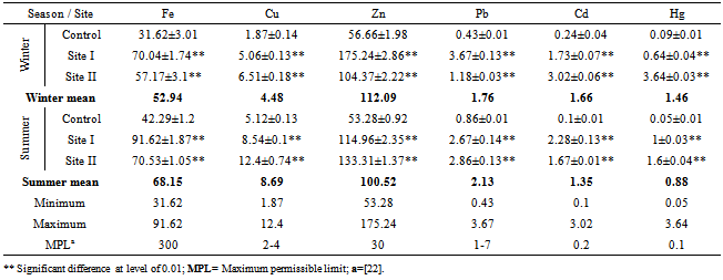
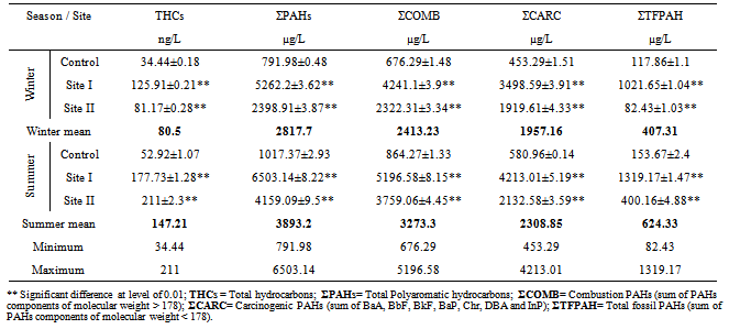
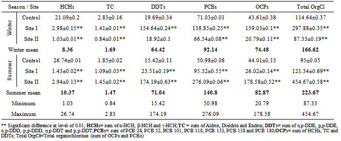
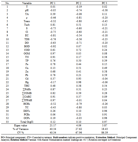
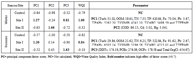
Water from the three sampling sites was examined for the physicochemical parameters during winter and summer of year 2011. The probability of average concentration for each parameter at each site was calculated and compared to the control site. Some marked variations in the parameters were observed between sampling sites and season, Table (2). There were significant variations in most of the physicochemical parameters for both seasons for sites I and II compared to the control site. However, waterdensity, transparency, salinity,chlorinity, electric conductivity (EC), total dissolved solids (TDS), biochemical oxygen demand (BOD5) and total phosphorus (TP) showed a highly significant increase (p≤0.01), while pH revealed no significant change. Also different significance change in temperature, total alkalinity (TA), turbidity, dissolved oxygen (DO), oxidizable organic matter (OOM)and total nitrogen (TN) were showed in Table (2). The control site recorded the highest mean value for temperature, pH, density, transparency, salinity, chlorinity, EC, TDS, DO and BOD5, while other parameters recorded the highest mean value in site I; TA, turbidity, COD, OOM, TN and TP. The lowest mean values for temperature, density, salinity, chlorinity, EC, TDS, DOand BOD5 were observed in site I, while that of pH and transparency were found in site II.Concentrations of the selected heavy metals were given in Table (3). Results showed significant increase (p≤0.01) in both sites I and II compared to the control site during both seasons for all studied metals. The average of heavy metals concentrations were in the following order: Zn>Fe>Cu>Pb>Cd>Hg. It has been noted that winter average for each of Zn, Cd and Hg was higher than that in summer, while summer average for each of Fe, Cu and Pb was higher than that of winter. Iron show a highly significant increase (p≤0.01) during both seasons with a seasonally average during summer lower than that in winter, showing maximum concentration at site Iduring summer and a minimum one at control site during winter. Cu showed maximum value in site II during summer, while its value was of minimum valueatthe control site during winter. Zn was the most abundant heavy metal in the present investigation, where it ranged between 53.28 ppb in the control site during summer to 175.24 ppb in site I during winter, both values in winter. The seasonally average during winter was higher than that during summer. Pbshowed the minimum and maximum values during winter. The seasonally average during winter was lower than that of summer. Cd showed a seasonal average during winter higher than that of summerand ranged between 0.10 ppb in the control site during summer to 3.02 ppb in site II during winter. Hgwas the least abundant heavy metal in the present investigation. Hg, like Cd, showed a minimum value in the control site during summer and a maximum value in site II during winter. The seasonally average during winter was higher than that during summer.Table (4) gives the total concentrations of total Hydrocarbons (THCs), as well as total Polyaromatic hydrocarbons (ΣPAHs), Combustion PAHs (ΣCOMB = sum of PAHs components of molecular weight >178), Carcinogenic PAHs (ΣCARC = sum of BaA, BbF, BkF, BaP, Chr, DBA and InP), Total Fossil PAHs (ΣTFPAH = sum of PAHs components of molecular weight <178)[21] which were measured in water. Generally all of these compounds showed significant increases (p≤0.01) during both seasons for both control and site I and revealed a higher summer average than that of winter. In the present study, the THCs concentrations varied from 34.44 to 211 µg/L, higher concentration occurred at site II during summer and the lower one was found for samples from the control site during winter. The seasonal average was 80.50 and 147.21 ppb in winter and summer respectively. ∑PAHs values ranged from 791.89 to 6503.14 ng/L. The highest concentration of total PAHs was recorded in water collected during summer from site I. Lower concentrations were detected in samples fromthe control site during winter. ∑PAHs varied seasonally showing higher summer average value (3893.20 ng/L), while its average concentration was (2817.70 ng/L) in winter. The sum of major combustion specific compounds (ΣCOMB) was ranged from 676.29ng/Lduring winter to 5196.58 ng/L during summer at site II. Similarly for the control and site II, ΣTFPAH ranged from 82.43 to 1319.17 ng/L during winter at site II and summer at site I respectively. The sum of carcinogenic PAHs (ΣCARC) was highest during summer at site I with a concentration of 4213.01 ng/L and was lowest (453.29 ng/L) during winter at the control site. Generally ΣCOMB> ΣCARC> ΣTFPAHfor all sites.Organochlorines contaminants including HCHs(α-, β- and γ-HCH), TC (Aldrin, dieldrin and endrin), DDTs (o,p´-DDE, o,p´-DDD, o,p´-DDT, p,p´-DDE, p,p´-DDD, p,p´-DDT) and PCBs including (PCB 28, 52, 101, 118, 153, 138 and 180) were determined in water. Table (5) is showing the concentrations of OCPs (sum of HCHs, TC and DDTs) and PCBs found in water collected at sampling sites, where the total organochlorines refers to the sum of PCBs and OCPs. Results revealed that average of individual compound concentration was in the following order: PCBs>DDTs>TC>HCHs and their seasonal average were higher in summer than that of winter. However, the maximum values recorded for HCHs, TC, DDTs and PCBs were 26.74, 2.83, 174.19 and 276.09 ng/L respectively, while the maximum values were 1.03, 0.84, 15.42 and 95.32 respectively. During winter, site II recorded the minimum HCHs, TC, OCPs and Total organochlorines values. Worthing to note that DDTs and PCBs concentrations in site II were significantly (p≤0.01) higher than those in other sites during summer. Although the control site was showed to have the maximum levels of HCHs and TC, but site II showed a high significance (p≤0.01) to be the highest loaded site with OCPs (178.58 ng/L) in summer. Total organochlorines concentrations varied from 87.33 to 454.68 ppb with seasonally average 166.62 and 223.67 ppb in winter and summer respectively. Higher concentration occurred at site II during summer with highly significant increase (p≤0.01). Lower concentration was found for samples from the same site (site II) in winter. The seasonally average of total organochlorines in winter (166.62 ng/L) recorded was lower than that of summer (223.67 ng/L).The output data revealed that three factors (PC1, PC2 and PC3) affected site pollution distribution, as`sociation and sources, with cumulative covariance of 86.39%. Varimax rotated components matrix is given in Table (6)to give an overview on the nature of loading among the parameters. PC1, PC2 and PC3 have Eigen values of 21.17, 4.06 and 3.87representing covariance of 40.34, 67.96 and 86.39%respectively. PC1 represented loading for Turbidity, OOM, TN, TP, Fe, Pb, ∑PAHs, ∑COMB, ∑CARC and ∑TFPAH. PC2 represented loading for COD, Cd and Hg. PC3 represented loading for DDTs, PCBs, OCPs and total organochlorines.For the evaluation of hot spot sites, principal component factorscores and WQI corresponding to each sitehad been evaluated, as indicated in Table (7). High values of principal component factor scores mean that this site is from hotspots and both of sites I and II could be considered as hot spots. Therefore, according to WQI values shown in Table (7) and Figure (2), sites could be arranged in order of decreasing pollution load as following: site I> site II>the control site. According to PCA data the origin of pollution corresponding to the hotspot sites (sites I and II) during both seasons are shown in Table (7). The origin of pollution at site I was mainly realated to PC1 in both seasons and to PC3 in summer only, while the origin of pollution at site II was related to PC2 in winter and PC3 in summer.Therefore, the drains receive agricultural and sewage drainage water. So, its salinity decrease progressively which affects greatly the biota, in addition, the exacerbation of eutrophication of the drains’ water that caused by the nutrient load from agricultural drainage water. As a result of extensive evaporation of water, progressive increase of salinity and accumulation of chemical pollutants (heavy metals, pesticides and other pollutants) is expected to change the quality the environment and cause detrimental effects to the aquatic life. Thus, the principal component analysis (PCA) used to define the natural variation of the above mentioned parameters by reduction of data to give a satisfactory evaluation. PCA was attempted for interpreting the data-set of 33 major water constituents and potentially toxic pollutants (Table 6).The cumulative Eigenvalue reaches >85.10%until the Factor 3. Factor loadings for Factor 1 to Factor 3 are compiled in Table (6), where large absolute values (>0.7) that indicate a reliable correlation is indicated by bold letters. Factor 1 includes Turbidity, OOM, TN, TP, Fe, Pb, ∑PAHs, ∑COMB, ∑CARC and ∑TFPAH which together constitute 40.34 %.Factor 2 (27.62 %) yields relatively large loadings for COD, Cd and Hg. Factor 3 (18.43 %) yields high loading for DDTs, PCBs, OCPs and Total Organochlorines. Site I was loaded with factor 1 (PC1) with nearly the same value of loading (1.27 and 1.30 in winter and summer respectively indicating that there was a continuous supply of Fe, Pb, ∑PAHs during both seasons in the discharged effluent contained in, beside the previous parameters; the origin of pollution could be related also to a disturbance in the turbidity, OOM, TN and TP values in this site. Whereas site II was highly affected by PC2 and PC3 in winter and summer respectively. Thus origin of pollution within this site was mainly heavy metals; Cd and Hg in winter, whereas the origin in summer was pesticidic components (DDTs, PCBs, OCPs and the Total organochlorine compounds), Table (7).Table (2). Physicochemical parameters, mean±SD, of water samples collected during 2011
 |
| |
|
Table (2). Continued
 |
| |
|
Table (3). Concentration of heavy metals (ppb), mean±SD,in water samples collected during 2011
 |
| |
|
Table (4). Concentrations of hydrocarbons, mean±SD, determined in water samples collected during 2011
 |
| |
|
Table (5). Concentration (ng/L)of Organochlorine pesticides (OCPs) and their individuals (HCHs, TC and DDTs) and Polychlorinated biphenyls (PCBs), mean±SD, in water samples collected during 2011
 |
| |
|
Table (6). Varimax rotated component matrix of water collected during 2011
 |
| |
|
Table (7). Principal component factor scores and water quality index (WQI) of water collected during 2011
 |
| |
|
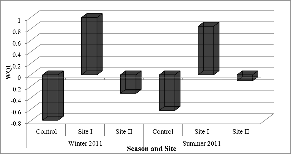 | Figure (2). Water quality index (WQI) values obtained from Principle component analysis (PCA) |
4. Study Conclusions
There were clear differences between the concentrations of detected heavy metals, hydrocarbons and organochlorinated compounds in water from the three sites.Generally higher concentrations were found during the summer compared to those detected during winter. WQI calculated in Table (7) revealed that sites could be arranged, from the highest polluted to lowest one, in the following order: Nubaria, Umoum then Kilo 21, Figure (2). Thus, Nubaria and Umoum drains were heavily loaded with these contaminants and they were the most highly polluted sampling sites and supposed to be hotspots of environmental pollutants due to industrial, agricultural and domestic wastes disposed and eluted compared to Kilo 21 drain which could be considered the control site for the present study.The analysis of variant species of pollutants is more advantageous than a single one, where PCA was helpful to reduce and extract the most effective groups of environmental pollutants and also to assign water quality within areas under investigation. Thus offers an effective early warning system for environmental monitoring programs.
References
| [1] | Basavaraja S., Hiremath S., Murthy K., Chandrashekarappa K., Patel A. and Puttiah E., (2011): Analysis of Water Quality Using Physico-Chemical Parameters Hosahalli Tank in Shimoga District, Karnataka, India. Global Journal of Science Frontier Research, 11 (3). |
| [2] | Saffran K., (2001): Canadian water quality guidelines for the protection of aquatic life, CCME water quality Index. User’s manual. Excerpt from Publication No.1299:ISBN1-896997- 34-1. |
| [3] | Sukarma T., Siddhartha C. and Priyanka T., (2011): Assessment of Water Quality of Ganga River in Kanpur by Using Principal Components Analysis. Advances in Applied Science Research, 2 (5):84-91. |
| [4] | Lohani B. and Todino G., (1984): Water Quality Index of Chao Phraya River. Journal of Environmental Engineering, 110 (6):1163-1176. |
| [5] | Shihab A., (1993): Application of Multivariate Method in the Interpretation of water Quality Monitoring Data of Saddam Dam Reservoir, Confidential 13. |
| [6] | Jayakumar R. and Siraz L., (1997): Factor analysis in hydro geochemistry of coastal aquifers – a preliminary study. Environmental Geochemistry, 31 (3/4):174–177. |
| [7] | Olobaniyi S., and Owoyemi F., (2006): Characterization by Factor Analysis of the Chemical Facies of Groundwater in the Deltaic Plain Sands Aquifer of Warri, Western Niger Delta, Nigeria. African Journal of Science and Technology (AJST), 7(1):73-81. |
| [8] | Canadian Council of Ministers of the Environment, (2011): Protocols manual for water quality sampling in canada. PN 1461, ISBN 978-1-896997- 7-0 PDF. |
| [9] | APHA, (1995): Standard methods for the examination of water and waste water; 19th ed. American Water Works Association and Water Pollution Control Federation Washington, DC. |
| [10] | APHA, (1992): Standard Methods for the Examination of Water and Waste Water; 18th ed., Academic Press. Broadway, Washington D.C. |
| [11] | USEPA, (1993): Methods for Determination of Inorganic Substances in Environmental Samples. EPA-600/R/93/100 - Draft. Environmental Monitoring Systems Lab., Cincinnati, Ohio. |
| [12] | Grasshoff K., (1976): Methods of Sea Water Analysis VCH. Weinheim, New York, pp. 31, 59, 97 and 117. |
| [13] | Strickland J. and Parsons T., (1975): A practical hand book of seawater analysis. Bulletin Fisheries Research Bd. Canada, Ottawa. |
| [14] | TrivedyR.,andGoel P., (1984): Chemical biological methods for water pollution studies. Env. Pub. Karad, India: pp.104. |
| [15] | FAO (Food and Agriculture Organization of the United Nations), (1975): Permanganate values of organic matter in natural waters. Fisheries Technical., 137: 169-171. |
| [16] | USEPA, (1978): Methods for the Chemical Analysis of Water and Wastes (MCAWW) (EPA/600/4-79/020). |
| [17] | Parsons T., Matia Y. and Malli G., (1985): “Determination of petroleum hydrocarbons”. A manual of chemical and biological method for seawater analysis, Pergamon Press, Oxford. |
| [18] | Sundberg H., Tjarnlund U., Akerman G., Blomberg M., Ishaq R., Grunder K., Hammar T., Broman D. and Balk L., (2005):The distribution and relative toxic potential of organic chemicals in a PCB contaminated bay. Marine Pollution Bulletin, 50: 195-207. |
| [19] | Astel A., Tsakovski S., Simeonov V., Reisenhofer E., Piselli S. and Barbieri P., (2008): Multivariate classification and modeling in surface water pollution estimation. Analytical and Bioanalytical Chemistry, 390 (5):1283-1292. |
| [20] | Saleh S., (2006): Environmental assessment of heavy metals pollution in bottom sediments from the Gulf of Aden, Yamen. Ph.D. Thesis, Institute of Graduate Studies and Research, Alexandria University, Egypt. 150 pp. |
| [21] | IARC, (1983): IARC monographs on the evaluation of the carcinogenic risk of chemicals to human. Polynuclear aromatic hydro- carbons, Part I, chemical, environmental, and experimental data. Agency for Research on Cancer, Lyons, 32: 1–477. |
| [22] | Environment Canada, (1987): Canadian Water Quality Guidelines [with updates]. Prepared by the Task Force on Water Quality Guidelines of the Canadian Council of Resource Ministers, Environment Canada, Ottawa |
 Abstract
 Reference
 Full-Text PDF
 Full-Text HTML