-
Paper Information
- Next Paper
- Previous Paper
- Paper Submission
-
Journal Information
- About This Journal
- Editorial Board
- Current Issue
- Archive
- Author Guidelines
- Contact Us
Resources and Environment
p-ISSN: 2163-2618 e-ISSN: 2163-2634
2012; 2(5): 228-239
doi: 10.5923/j.re.20120205.06
Studies on Meteorological Parameters and Mixing Height in Gold Mining Area
 Abstract
 Reference
 Full-Text PDF
 Full-Text HTML
Surendra Roy 1, Piyush Gupta 2, Trilok Nath Singh 3
1JCDM College of Engineering, Sirsa, 125055, Haryana, India
2National Institute of Rock Mechanics, Kolar Gold Fields, 563117, Karnataka, India
3Indian Institute of Technology, Bombay, 400076, Maharashtra, India
Correspondence to: Surendra Roy , JCDM College of Engineering, Sirsa, 125055, Haryana, India.
| Email: |  |
Copyright © 2012 Scientific & Academic Publishing. All Rights Reserved.
Gold mining at Kolar Gold Fields is closed but some industries in this area are in operation and some may like to be established. Data on atmospheric and meteorological parameters were generated using SODAR (Sound Detection and Ranging) and automatic weather station in different seasons. Over 2000 sodar echograms were recorded and classified into six categories like rising layer, thermal plume (free), ground based layer (spiky top), ground based layer (flat top), ground based multiple layers and dot echo structures. Using echograms, unstable period was determined to know the diluting capability of atmosphere for pollutants in the seasons. The highest duration of mixing heights revealed the period of highest dispersion. Based on the sodar echograms and mixing height, stability classes for the different times of the day were evaluated, which can be used for the estimation of dispersion coefficients. Influence of wind speed, wind direction, temperature, humidity, solar radiation and rainfall on mixing heights was studied. Statistical model was developed for the prediction of mixing height. Model adequacy was checked using F-statistics, normal distribution curve and correlation between predicted and measured values of mixing heights.
Keywords: Kolar Gold Fields, Meteorological Parameters, Mixing Height, Sodar, Weather Station, Stability Classes
Article Outline
1. Introduction
- The concentration of atmospheric pollutants is affected by atmospheric flows and by dispersion within the atmospheric boundary layer (ABL). ABL, being the lower part of the troposphere, is governed by the influence of the earth’s surface through friction, convective heating during the day, and radiative cooling of the ground during the night[1]. The height of the atmospheric boundary layer (ABL) or mixing height (MH) is a fundamental parameter that characterizes the structure of the lower atmosphere. Mixing height determines the volume available for the dispersion of pollutants by convection or mechanical turbulence and it is used in environmental monitoring and prediction of air pollution[2-5]. Topographical features and climatological conditions also influence the mixing height and evolution of stable and unstable ABL. The use of mixing height data of one particular site for another will be unjust and unwise when dealing with the dispersion models which require site-specific mixing height and stability class data[6]. In addition to latitudinal variation[7], meteorological parame ters may also affect the mixing height. Spurr[8] stated that the pollutants discharged into the atmosphere depend upon the meteorological conditions prevailing in the earth’s atmospheric boundary layer. Kolar Gold Fields is located in Karnataka, India where gold mining was carried out over 120 years. The mine is closed since January 2000[9]. But some industries are in operation and some may likely to be established in near future. As the dissipation of air pollutants in vertical and lateral directions depends basically on atmospheric and meteorological conditions, therefore, study on these parameters will be helpful for the industries either in operation or to be set up in this area to reduce their impacts. Considering these, seasonal data on atmospheric and meteorological parameters were generated for the assessment of stability periods, to find out the seasonal variation in mixing height, to determine the stability classes of the area, to study the influence of meteorological parameters on mixing height, and to develop statistical model for the evaluation of mixing height.
2. Data Generation Using Sodar and Automatic Weather Station
- SODAR stands for sound detection and ranging. A tri-axis monostatic (back-scattering) sodar, manufactured by Global Environmental Technologies, New Delhi, India, with a technical know-how of the National Physical Laboratory, New Delhi, India, was installed at the roof of office building of National Institute of Rock Mechanics, Kolar Gold Fields, India. The automatic weather station of Lawrence & Mayo (India) Pvt. Ltd. was installed adjacent to sodar. Sodar was operated continuously for 24-hours in winter (February), summer (May), monsoon (August) and post-monsoon (November) for a period of 27, 29, 31 and 17 days respectively. Weather station was also operated in corresponding months of the seasons. The working principle of sodar and weather station has been explained in Roy et al.[10].
3. Results and Discussion
3.1. Categorisation of Sodar Echograms
- Over 2000 sodar echograms recorded in different seasons were analysed and classified into different categories. Though there were some variations in the echogram structures, the observed echograms were broadly classified into six categories as shown in Figure 1.Figure 1a shows the rising echograms which occur in the morning some time after sunrise. The rising echograms indicate transition from stable to unstable conditions. Such echograms were observed late in winter than in other seasons. The incoming solar radiations gradually erase the ground based temperature inversion layer. With continuous solar heating, the layer starts rising, indicating the transfer of heat, momentum and energy from the earth’s surface [11-13]. In winter, convection period started late due to low surface heating[14].Figure 1b exhibits the thermal plume (free) types of echograms which were observed during the day time i.e. strong convection periods up to 16:00 IST (Indian Standard Time). Thermal plumes (free) or convective conditions are caused by turbulence in the unstable condition (temperature decreases with height) and its strength become maximum in the afternoon[11] or at noon[12] and then decreases with the fall in solar heat flux[11-12]. The strong convection period is followed by weak convection, which persists till sunset.Ground based spiky top layers were observed (Figure 1c) in the evening. Often the presence of winds during temperature inversion is responsible for this type of structures. Under this situation, the wind tends to cause instability in temperature inversion layers[13]. Ground based flat top layers (Figure 1d) were found during clear weather after midnight. When the heating due to radiation stops in the evening, cooling of earth surface establishes a stable boundary layer[15]. Owing to large radiative cooling at ground surface, a nocturnal stable boundary layer forms after sunset and persist throughout the night[12]. Very stable situations are usually associated with clear nocturnal skies and weak winds or with the advection of warm air over a much cooler surface[16]. Flat top layers are formed on clear nights (associated with very light wind conditions)[13] due to emission of infrared radiations from the ground. Singal et al.[11] observed flat top layers under slight or no wind conditions during night time. The thickness of these layers may increase with time.Ground based multiple layers (Figure 1e) also occurred after midnight when temperature increases with height. Light wind conditions or advection are responsible for these types of layers[3, 11]. Katabatic winds during the radiative cooling of ground also form layered structures[17].
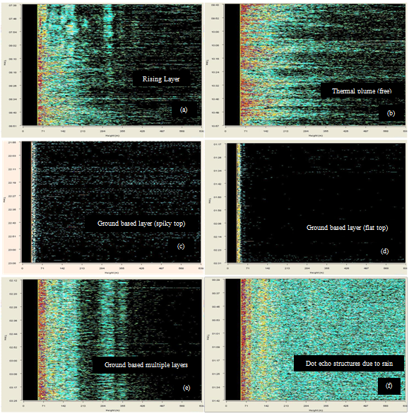 | Figure 1. Typical sodar echograms at the site |
3.2. Assessment of Stability Periods Using Sodar Echograms
- Based on the observations of sodar echograms, onset and dissipation time of convective boundary layer was ascertained. Table 1 shows that onset time of convective boundary layer is late by an hour in winter than in other seasons. As the days are shorter in winter, the duration of convective period is the minimum in this season. The dissipation time is same for all the seasons. The duration of convective activity is the lowest in winter. Depending on seasons, there was variation in onset and dissipation time and hence duration of convective activity. The convective activity during day time determines the atmospheric boundary layer’s diluting capability for pollutants[6].The duration of convective activity is called unstable period while remaining hours are called stable period. The relative occurrence of unstable and stable periods in different seasons was determined (Figure 2). The occurrence of unstable period was the lowest in winter and corresponding stable period was the highest in this season compared to other seasons.
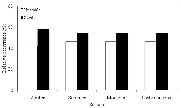 | Figure 2. Seasonal variation in unstable and stable periods |
| |||||||||||||||||||||||||||||||||||||||||||||||||||||||||||
3.3. Mixing Height
- Mixing height is defined as the height of the layer adjacent to the ground over which pollutants enter into this layer get mixed up by convection or mechanical turbulence within one hour[3, 20] or it is the height above the surface up to which emitted air pollutants are diluted[21]. It is a fundamental parameter that characterizes the structure of the lower atmosphere and determines the volume available for dispersion of pollutants by convection or mechanical turbulence[2, 3, 4, 5, 17, 20, 22, 23]. Higher the mixing height, the higher is the volume available for the dispersion of pollutants and vice versa. The stable boundary layer is indeed quite shallow compared to convective boundary layer or unstable boundary layer[24]. The structure of the atmospheric boundary layer is determined by various processes (turbulence, radiation, baroclinity, advection, divergence and associated vertical motion, etc.) which influence the vertical profiles and turbulent atmospheric parameters in a different way especially in the stable boundary layer[3].The mixing height was determined using the method given in Roy et al.[10]. Hourly variation in mixing height for different seasons is shown in Figure 3. Mixing height is low during stable boundary layer and high in between 12:00 IST and 14:00 IST in all the seasons. After 16:00 IST, the mixing height starts decreasing due to lower heating of the ground. The majority of mixing heights during transition phase (stable to unstable and vice versa) were within 650 m in all the seasons. Even during weak convection, which occurred before sunset, the mixing height was also within 650 m. The highest mixing height during convection period was 2785 m, 2606 m, 2307 m, and 1189 m in winter, summer, monsoon, and post-monsoon respectively. Mixing heights were highest between 12:00 IST and 14:00 IST due to highest convection during this period in all the seasons[11, 14]. According to Gera et al.[7], lower latitudes receive more solar energy due to higher solar zenith angle compared to higher latitudes. Hence lower latitude causes higher mixing height than higher latitude. The lower latitude (12056’17.93’’) at Kolar Gold Fields might be the reasons for higher mixing heights in the seasons.
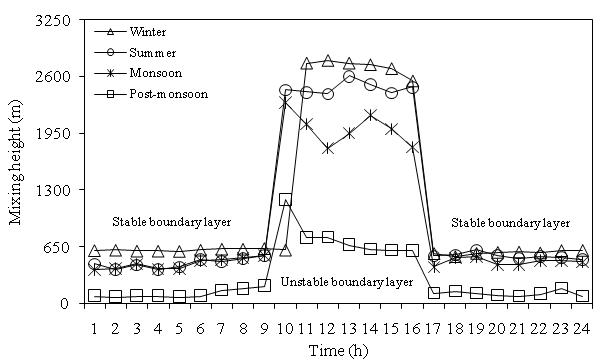 | Figure 3. Seasonal variation in mixing height |
3.4. Determination of Stability Classes
- Atmospheric stability is one of the essential parameters for air quality studies. Among Pasquill[25] stability classes, the presence of class A indicates strong mixing whereas E or F gives rise to poor dispersion[26-27]. The stability classes can be determined based on mixing heights and sodar echograms[6, 11]. Using sodar echograms and corresponding mixing heights[10, 28], stability classes for the site condition were determined. Classes A, B, C was found during convection periods of the days in the seasons. In the evening, class E was considered due to low infrared radiation and spiky top layers. After midnight, ground based flat top and multiple layers echograms or mixing height above 100 m indicated class F. Class D was absent as no echogram structures (blank) or zero mixing height were observed. Table 2 summarizes stability classes for different periods of the day for different seasons. Class A was predominant during 09:00-16:00 IST in summer and monsoon whereas during 10:00-16:00 IST in winter. In post-monsoon, class B was predominant during 9:00-16:00 IST. These periods fall under strong convection period of the day. Class B also occurred during weak convection period of the day i.e. at 08:00-10:00 IST in winter and at 07:00-09:00 IST in summer and monsoon. It was also observed at 16:00-18:00 IST in all the seasons except in post-monsoon. Class C was found at 07:00-09:00 IST and 16:00-18:00 IST in post-monsoon. Class E occurred in the evening and F in the morning in the seasons. The Pasquill stability classes can be used to determine the horizontal and vertical dispersion coefficients as a function of downwind distances from the source using Pasquill-Gifford curves[11, 29]. These coefficients can be used to calculate emission rate for the industries either in operation or likely to be set up in this area.
3.5. Influence of Meteorological Parameters on Mixing Height
- Meteorological parameters such as wind speed, wind direction, surface temperature, humidity, solar radiation and rainfall can affect the mixing height. Therefore, the influence of these parameters on mixing height was studied.The meteorological data generated for each season were analysed. Though the number of monitoring days for meteorological parameters compared to operation periods of the sodar was more in some seasons, only those meteorological data corresponding to mixing height were considered for analysis. The hourly average values of meteorological parameters and mixing height for different days of different seasons were calculated separately. Hence, hourly data for each season was used for analysis.
3.5.1. Wind Speed and Direction
- The change of wind direction and speed with time at a particular site can be presented diagrammatically in the form of a wind rose. A wind rose diagram consists of a series of lines emanating from the centre of a circle and pointing in the direction from which the wind blows. It shows the prevailing wind direction and speed. The length of the bar for a direction indicates the percent of time the wind comes from that direction. The percentage of time for velocity is shown by the thickness of the direction bar. The circle marked in the centre of the wind rose indicates the percent of time covered for calms with very low wind velocities. Wind rose diagrams (Figure 4) were plotted for all seasons using hourly data of wind speed and direction with the help of ISC – AERMOD View software version 5.9. The level of frequencies (%) is mentioned on each circle through which frequency for each direction can be assessed. In winter (Figure 4a), the highest percentage of winds was from W at a speed up to 8.8 m/s. The calm conditions were 21.13 % of the time. In summer (Figure 4b), the percentage of winds was the highest from NW up to 8.8 m/s. The wind also blew up to this speed from other directions. The calm period was 18.89% of the time in this season. In monsoon (Figure 4c), the highest percentage of wind was from WNW. The wind blew from different directions up to 8.8 m/s in this season. The percentage of calm condition was 4.17%. In post-monsoon, the wind rose (Figure 4d) indicates that the greatest percentage of wind blew from W at a speed of up to 8.8 m/s. The calm conditions prevailed 22.27 % of the time. The directions of the resultant unit vector for different seasons are also shown in the Figure. It is a common way to represent the mean wind direction. The magnitude of the resultant vector for the wind rose represents the frequency count for the mean direction.The calm condition was the highest in post-monsoon and the lowest in monsoon indicating the wind blew more in monsoon and less in post-monsoon. Generally the plume of the air pollution from the industries moves towards the downwind direction. If the wind direction is constant, the area remains exposed to high pollutant levels. As the direction changes, pollutant disperse over a large area causing lower concentrations over the exposed area. The predominant wind directions in different seasons can help in the design of greenbelts of fast growing trees to minimize the environmental impacts of industries. Good correlation of wind speed with mixing height for different seasons (Figure 5) shows the influence of wind speed on mixing height. In the Figures, N indicates number of monitoring days in the season. Using SPSS software version 13.0, the significant level of correlation coefficients was checked and it was found that correlations are statistically significant at 1% level of significance except summer. Positive correlation indicates that as the wind speed increases mixing height increases. These results agree with those published by Roy et al.[10], Singal et al.[11] and Zhou et al.[23]. Using the monitored data, wind direction was plotted against mixing height for different seasons and analysed (Figure 6). Correlations were statistically significant at 5% level of significance in the seasons except monsoon. Limited variations of wind direction in monsoon might be the reason for poor correlation.
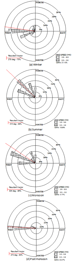 | Figure 4. Windrose diagrams (a) winter (b) summer (c) monsoon and (d) post-monsoon |
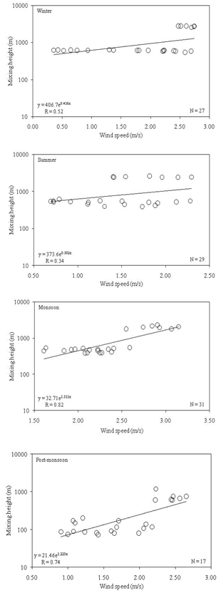 | Figure 5. Correlation of wind speed with mixing height in different seasons |
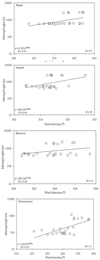 | Figure 6. Correlation of wind direction with mixing height in different seasons |
3.5.2. Temperature
 | Figure 7. Hourly variation in temperature in different seasons |
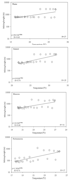 | Figure 8. Correlation of temperature with mixing height in different seasons |
3.5.3. Humidity
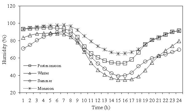 | Figure 9. Hourly variation in humidity in different seasons |
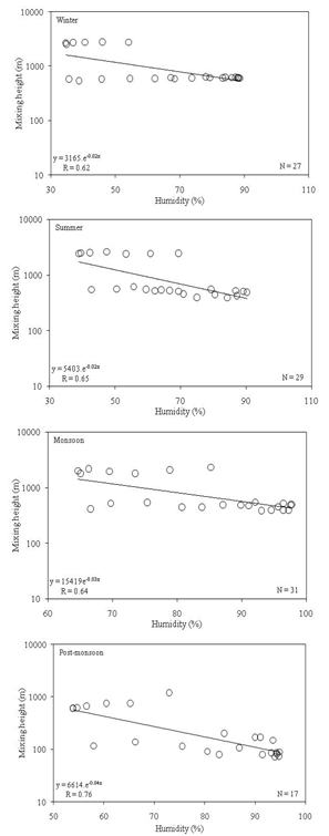 | Figure 10. Correlation of humidity with mixing height in different seasons |
3.5.4. Solar Radiation
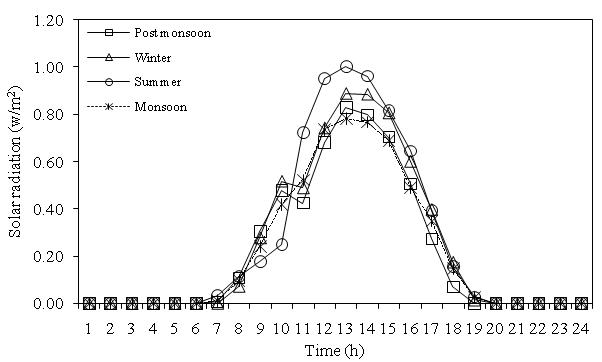 | Figure 11. Hourly variation in solar radiation in different seasons |
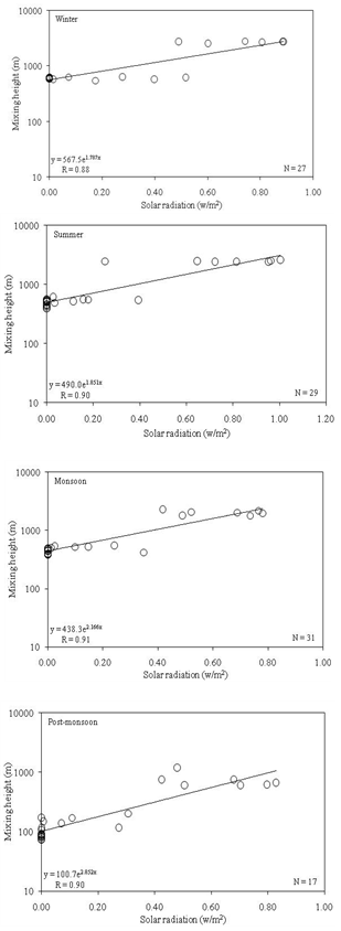 | Figure 12. Correlation of solar radiation with mixing height in different seasons |
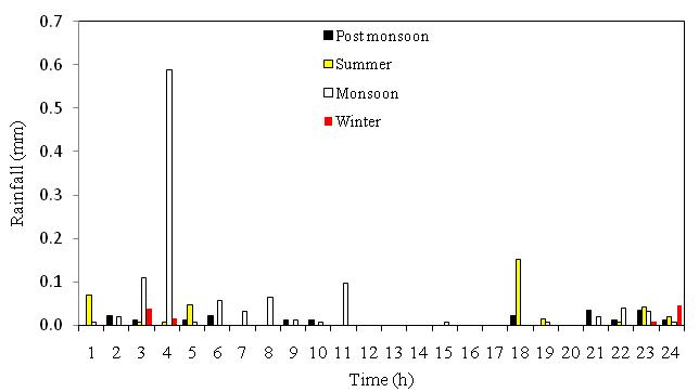
3.5.5. Rainfall
- Rainfall occurred in all the seasons. The recorded rainfall for different seasons is shown in Figure 13. Using the monitored data, mixing height was plotted against rainfall (Figure 14). Variations in rainfall at different periods of the days might have led to variations in infrared cooling of the earth. This could be the reason of insignificant influence on mixing height.
 | Figure 13. Hourly variation in rainfall in different seasons |
3.5.6. Multiple Regression Analysis of Data
- Individual correlation of meteorological parameters with mixing height indicated that some are significantly correlated and some are not. Therefore, all the parameters were combined and step wise regression analysis of data was carried out to select the actual subset of the variables influencing the mixing height i.e. developing the model for predicting the mixing height. Generally, for most of the practical problems, there are many predictors which include all the influential factors, but the actual subset of predictors that should be used in the model needs to be determined. Finding an appropriate subset of regressors for the model is called the variable selection[31]. According to different researchers[32-34], stepwise multiple regression procedure is commonly used to produce a parsimonious model that maximizes accuracy with an optionally reduced number of predictor variables.To develop statistical models, multiple regression analysis of 96 sets of data consisting of 24 sets for each season was carried out using the SPSS software version 13.0. With the help of stepwise regression procedure, two models were developed (Tables 4). The adjusted R2 value is the highest and the residual mean square is the lowest for model 2. The derived regression coefficients are neither zero nor less than the standard error. For a model, adjusted R2 increases if the addition of the variable reduces the residual mean square. In addition, it is not good to retain negligible variables, that is, variables with zero coefficients or the coefficients less than their corresponding standard errors[31]. Variance inflation factor (VIF) for the input variables is lower than 10 indicating that there is no multicollinearity[31] as higher values cause poor prediction equations.
| ||||||||||||||||||||||||||||||||
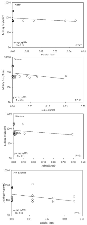 | Figure 14. Correlation of rainfall with mixing height in different seasons |
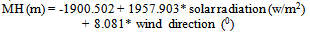 | (1) |
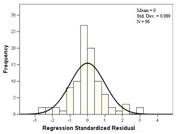 | Figure 15. Standardized residual analysis of mixing height model |
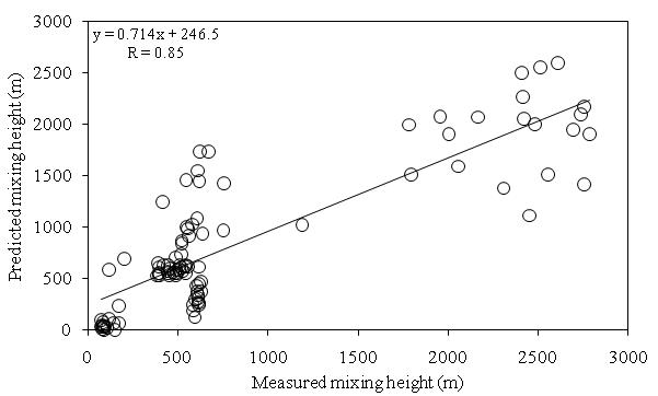 | Figure 16. Correlation between predicted and measured values of mixing height |
4. Conclusions
- Based on the study of atmospheric and meteorological parameters, the unstable period for summer, monsoon and post-monsoon is from 7:00 to 18:00 IST whereas for winter it is from 8:00 to 18:00 IST indicating that emission of pollutants during these periods from the industries either in operation or likely to be established in this area will have less impacts on surrounding habitations. The mixing height was the highest between 12:00 IST and 14:00 IST in all the seasons indicating the highest volume of air will be available for the dispersion of pollutants during this period. Stability classes A, B, C, E and F were predominant at different times of the day in the seasons. These classes can be used to find out the dispersion coefficients required for the computation of emission rates of pollutants. The predominant wind direction as indicated by windrose diagrams for different seasons can be used to minimise the impacts of air pollution by planting fast growing trees perpendicular to the plume moving towards habitations. Simple correlations of meteorological parameters with mixing height showed different degree of correlations. Step wise regression analysis of data revealed that solar radiation and wind direction significantly influence the mixing height. The performance of the developed statistical model indicated that it can be used to predict mixing height for the study area.
ACKNOWLEDGEMENTS
- The facilities availed during my services at the National Institute of Rock Mechanics is gratefully acknowledged.
References
| [1] | Dayan, U. and Rodnizki, J., 1999, The temporal behavior of the atmospheric boundary layer in Israel., J. Appl. Meteorol., 38 (6), 830-836. |
| [2] | Aron, R., 1983, Mixing height – an inconsistent indicator of potential air pollution concentrations., Atmos. Environ., 17 (11), 2193-2197. |
| [3] | Beyrich, F., 1997, Mixing height estimation from sodar data – a critical discussion., Atmos. Environ., 31 (23), 3941-3953. |
| [4] | Aksakal, A., 2001, Sodar studies of the mixing height in the Arbian Gulf coast region., Arab. J. Sci. Eng., 26, 23-32. |
| [5] | Eresmaa, N., Karppinen, A., Joffre, S.M., Rasanen, J. and Talvitie, H., 2005, Mixing height determination by Ceilometer., Atmos. Chem. Phys. Discuss., 5, 12697-12722. |
| [6] | Gera, B.S. and Saxena, N., 1996, Sodar data – a useful input for dispersion modeling., Atmos. Environ., 30 (21), 3623-3631. |
| [7] | Gera, N., Gupta, N.C., Gera, B.S., Mohanan, V., Gupta, P.K., Singh, N., Malik, J., Singh, G. and Ojha, V.K., 2008, Latitudinal variation of mixing height over Delhi-Hyderabad Corridor., Available: rp.iszf.irk.ru/hawk/URSI2008/paper/FP2p9.pdf. |
| [8] | G. Spurr, Meteorological Factors and Dispersion. In: Indusial Air Pollution Handbook (ed. A. Parker), McGraw-Hill Book Company (UK) Limited, England, pp. 123-141, 1978. |
| [9] | Rao, S.M., and Reddy, B.V.V., 2006, Characterization of Kolar gold field mine tailings for cyanide and acid drainage., Geotech. Geol. Eng., 24 (6), 1545-1559. |
| [10] | Roy, S., Adhikari, G.R., Renaldy T.A. and Singh T.N., 2011, Assessment of atmospheric and meteorological parameters for control of blasting dust at an Indian large surface coal mine., Res. J. Environ. Earth Sci., 3(3), 234-248. |
| [11] | S.P. Singal, B.S. Gera and N. Saxena, Sodar: A Tool to Characterize Hazardous Situations in Air Pollution and Communication. In: Acoustic Remote Sensing Applications (ed. S.P. Singal), Narosa Publishing House, New Delhi, India, pp 326-384, 1997. |
| [12] | Nilsson, E.D., Rannik, U., Kulmala, M., Buzorius, G. and O’Dowd, C. D., 2001, Effects of continental boundary layer evolution, convection, turbulence and entrainment, on aerosol formation., Tellus, 53B, 441-461. |
| [13] | Choudhury, S. and Mitra, S., 2004, A connectionist approach to SODAR pattern classification., IEEE Geosci. Remote Sens. Lett., 1 (2), 42-46. |
| [14] | Myrick, R.H., Sakiyama, S.K., Angle, R.P. and Sandhu, H.S., 1994, Seasonal mixing heights and inversions at Edmonton, Alberta., Atmos. Environ., 28 (4), 723-729. |
| [15] | J.C. Mayer, Characterisation of the Atmospheric Boundary Layer in a Complex Terrainusing SODAR-RASS., Diploma thesis in Geoecology, Department of Micrometeorology, University of Bayreuth, Germany, 2005. |
| [16] | Mahrt, L., 1999, Stratified atmospheric boundary layers, Bound.-Lay. Meteorol., 90, 375-396. |
| [17] | Garcia, M.A., Sanchez, M.L., De Torre, B. and Perez, I.A., 2007, Characterisation of the mixing height temporal evolution by means of a laser dial system in an urban area – intercomparison results with a model application., Ann. Geophys., 25, 2119-2124. |
| [18] | Gera, B.S. and Singal, S.P., 1990,Typical boundary layer studies during monsoon period using Sodar., Proc., 5th International Symposium on Acoustic Remote Sensing of the Atmosphere and Oceans, 6-9 February, New Delhi, pp. 390-394. |
| [19] | Singal, S.P., Gera, B.S. and Aggarwal, S.K., 1985, Studies of sodar-observed dot echo structures., Atmos. Ocean, 23 (3), 304-312. |
| [20] | Seibert, P., Beyrich, F., Sven-Erik, G., Joffre, S., Rasmussen, A. and Tercier, P., 2000, Review and intercomparison of operational methods for the determination of the mixing height., Atmos. Environ., 34, 1001-1027. |
| [21] | Tombrou, M., Dandou, A., Helmis, C., Akylas, E., Angelopoulos, G., Flocas, H., Assimakopoulos, V. and Soulakellis, N., 2007, Model evaluation of the atmospheric boundary layer and mixed-layer evolution., Bound.-Lay. Meteorol., 124, 61-79. |
| [22] | Baars, H., Ansmann, A., Engelmann, R. and Althausen, D., 2008, Continuous monitoring of the boundary-layer top with lidar., Atmos. Chem. Phys. Discuss., 8, 10749-10790. |
| [23] | Zhou, B., Yang, S.N., Wang, S.S. and Wagner, T., 2009, Determination of an effective trace gas mixing height by differential optical absorption spectroscopy (DOAS)., Atmos. Meas. Techn., 2, 1663-1692. |
| [24] | Nieuwstadt, F.T.M. and Duynkerke, P.G., 1996, Turbulence in the atmospheric boundary layer., Atmos. Res., 40, 111-142. |
| [25] | Pasquill, F., 1961, The estimation of the dispersion of wind borne material., Meteorol. Mag., 90, 34-49. |
| [26] | L.W. Canter, Environmental Impact Assessment, McGraw-Hill Book Company, New York, p. 77, 1977. |
| [27] | R.A. Dobbins, Atmospheric Motion and Air Pollution, John Wiley & Sons, New York, p. 224, 1979. |
| [28] | Operational Manual, SODAR, Global Environmental Technologies, New Delhi, India, 2008. |
| [29] | Gifford, F.A., 1961, Use of routine meteorological observations for estimating atmospheric dispersion., Nucl. Saf., 2, 47-51. |
| [30] | Gera, B.S., Singal, S.P. and Ojha, V.K., 1990, Sodar studies of the boundary layer during a synoptic fog storm., 5th International Symposium on Acoustic Remote Sensing of the Atmosphere and Oceans, 6-9 February, New Delhi, pp. 429-435. |
| [31] | D.C. Montgomery, E.A. Peck and G.G. Vining, Introduction to Linear Regression Analysis, John Wiley & Sons, Inc., New York, 2003. |
| [32] | Comrie, A.C., 1997, Comparing neural networks and regression models for Ozone forecasting., J Air Waste Manag Assoc., 47, 653-663. |
| [33] | Chaloulakou, A., Grivas, G. and Spyrellis, N., 2003, Neural network and multiple regression models for PM10 prediction in Anthens: A comparative assessment., J Air Waste Manag Assoc., 53, 1183-1190. |
| [34] | Grivas, G. and Chaloulakou, A., 2006, Artificial neural network for prediction of PM10 hourly concentrations, in the Greater Area of Athens, Greece., Atmos. Environ., 40, 1216-1229. |
| [35] | Goyal, P., Chan, A.T. and Jaiswal, N., 2006, Statistical models for the prediction of respirable suspended particulate matter in urban cities., Atmos. Environ., 40, 2068-2077. |
| [36] | Papanastasiou, D.K., Melas, D. and Kioutsioukis, I., 2007, Development and assessment of neural network and multiple regression models in order to predict PM10 levels in a medium-sized Mediterranean city., Water Air Soil Pollut., 182, 325-334. |