-
Paper Information
- Previous Paper
- Paper Submission
-
Journal Information
- About This Journal
- Editorial Board
- Current Issue
- Archive
- Author Guidelines
- Contact Us
Resources and Environment
p-ISSN: 2163-2618 e-ISSN: 2163-2634
2012; 2(2): 30-36
doi: 10.5923/j.re.20120202.05
Prediction of Particulate Matter Concentrations Using Artificial Neural Network
Surendra Roy
National Institute of Rock Mechanics, Kolar Gold Fields, Karnataka, 563117, India
Correspondence to: Surendra Roy , National Institute of Rock Mechanics, Kolar Gold Fields, Karnataka, 563117, India.
| Email: |  |
Copyright © 2012 Scientific & Academic Publishing. All Rights Reserved.
Mill tailings at Kolar Gold Fields are creating particulate pollution on air environment. In the previous study, multiple regression models were developed for the prediction of particulate matter concentrations using data of meteorological parameters (wind speed, wind direction, temperature, humidity and solar radiation) and particulate matter (PM10 and TSP) monitored in different seasons[1]. Artificial neural network is an excellent predictive and data analysis tool for the evaluation of air pollutants. Therefore, the data were used for the development of neural network models. During development of models, the values 0.02, 0.5 and 0.7 were used as target error, learning rate and momentum respectively. Three hidden layers were used to obtain acceptable values. Performance of the models was evaluated using those sets of data which were not used during learning of neural network. Architecture of developed networks, number of hidden neurons and weights, normalised and relative error, importance and sensitivity, etc have been discussed in this paper.
Keywords: Neural networks, Particulate matter, Meteorological parameters, Gold mill tailings, Kolar Gold Fields
Article Outline
1. Introduction
- Nowadays, there is almost unanimous scientific consensus that air quality degradation is one of the major environmental hazards in many areas and a lot of research is therefore conducted in the field of air pollution. The forecasting of the airborne particulate matter concentrations is of particular interest due to its well known adverse health impact to humans[2]. In the previous study, multiple regressions analysis of data was carried out to develop the statistical equations for the prediction of PM10 and TSP[1]. Different researchers have developed several statistical techniques, artificial neural networks (ANN) are expected to show better particle forecasting performance when compared to the traditional ones (e.g. regression models). This is because they have the better adaptation ability on fitting data to describe highly nonlinear physical processes[2]. The artificial neural network models has been used to predict different air pollutants like atmospheric sulphur dioxide, nitrogen oxides and particulate matter[3- 5]. Compared to atmospheric modeling systems, it requires limited input data and computer power[6] and provides a highly effective tool to model atmospheric dispersion[7]. Therefore, using the data generated, neural network models have been developed to predict PM10 and TSP concentrations in the study area.
2. Methodology
2.1. Monitoring Station and Data Generation
- Monitoring was carried out at the National Institute of Rock Mechanics (NIRM), Kolar Gold Fields (KGF). Details of monitoring station, particulate and meteorological measurements have been explained in Roy and Adhikari[1].
2.2. Artificial Neural Network
- The artificial neural networks arise as a mechanism to mimic the human brain’s processes. Its objective is to compute output values from input data by some internal calculations. In fact, this method based on a highly interconnected system and a simple processing element (known as neuron), which can learn the interrelationship between independent and dependent variables[8]. The most popular ANN is the multi-layer feed-forward neural network, where the neurons are arranged into layers of input, hidden and output. Feed-forward neural network usually has one or more hidden layers, which enable the network to model non-linear and complex functions. Each neuron consists of a transfer function expressing internal activation level. Output from a neuron is determined by transforming its input using a suitable transfer function. Transfer functions may be linear or non-linear. Sigmoidal function is commonly employed for non-linear relationship. The most popular transfer function is the logarithmic sigmoid. The sigmoid function is bounded between 0 and 1, so the input and output data should be normalized to the same range as the transfer function used. Normalisation of inputs leads to avoidance of numerical overflows due to very large or very small weights[9].Among possible neural net simulators available like Matlab, WEKA and EasyNN, many researchers have used Matlab for the prediction of air pollutants. In this study, EasyNN-plus software was used for the development of ANN model. This software is easiest in use, simplifies many of the steps needed for creating simple and efficient neural network models[10]. The EasyNN-plus package uses a back-propagation algorithm and a sigmoidal function to build the models. The data needed for training the network can be generated with simple text or spreadsheet software. In addition, the program can either assume values for the learning rate and momentum or let it up to the user. After the models are built, they can be used for estimating output values[11]. According to Razavi et al.[9], it is simple to build a network for modelling and prediction with EasyNN.
3. Model Development and Evaluation
- The meteorological data were downloaded to the computer once in a month. Though these data were generated for about one year, the data used in this study correspond to the dust monitoring period. As meteorological parameters such as wind speed, wind direction, temperature, humidity and solar radiation influences the particulate concentrations, therefore, considering TSP and PM10 as dependent and meteorological parameters as independent variables, a total of 72 sets of data, consisting of 24 sets for each season, were used for the models development[1]. Out of 72 data sets, 70 sets were used for training the network and 2 sets for querying. The training data was used for learning the ANN whereas the querying data was used to test the neural networks predictability.
 | Figure 1. Architecture of network for (a) PM10 and (b) TSP (input, three hidden and output layers) |
3.1. Architecture of Network for Particulate Assessment
- Before training or learning started, all the sets of data were checked for conflict. No any conflict was observed in any set of data indicating that monitored data are suitable for training purpose. During training, software assigns a weightage to various inter-related parameters and attempts to limit the error. This process is repeated until the error converges to the set limits. The final weightages are obtained after training[12]. For learning the network, the target error value was set to 0.02. The control of learning was stopped when all the errors were below the target value. The learning rate and momentum was set to 0.5 and 0.7 respectively. The network developed for PM10 consisted of 5 inputs (wind speed, wind direction, temperature, humidity and solar radiation), 19 hidden (3 layer system) and 1 output neuron (PM10). In TSP neural network, the input parameters were same as PM10 but 3 hidden layers consisted of total 29 neurons. For both the particulate, the architecture was below the targeted error (Figure 1a, b). As acceptable results occurred with three hidden layers; therefore, three hidden layers were used in the network[13, 12]. The thickness of the connections represented the weights of different processing elements.
3.2. Cycles and Errors Status of Networks
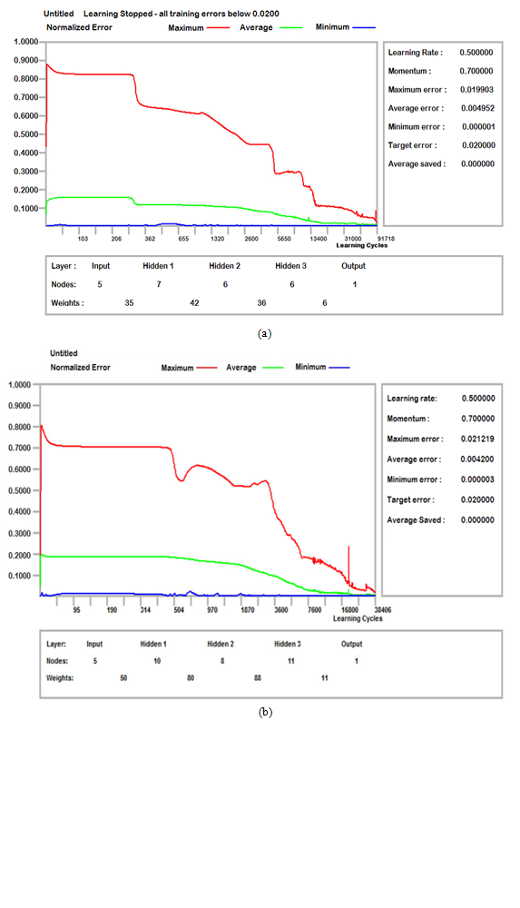
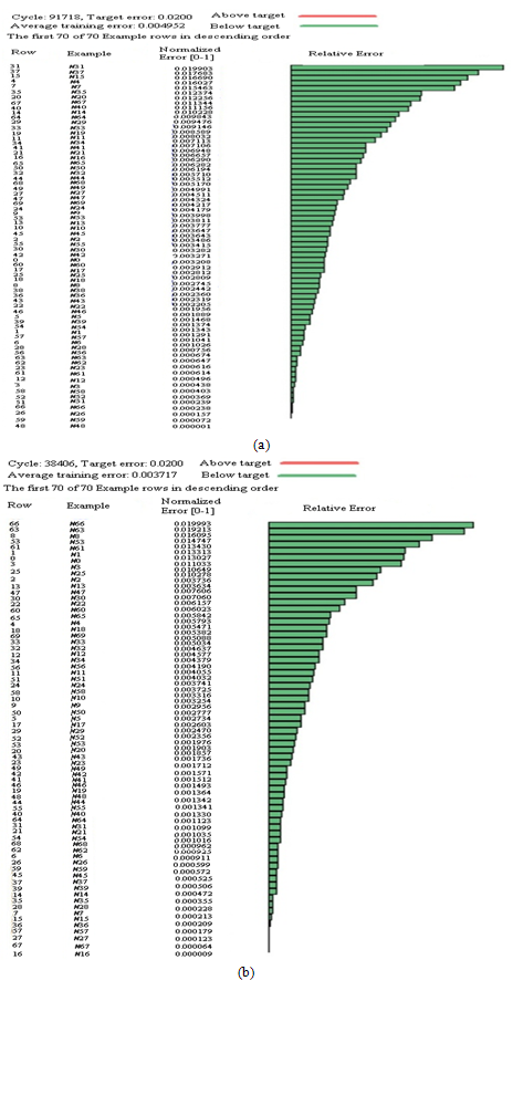
- The learning of PM10 and TSP was completed after 91718 and 38406 cycles respectively. The weights of the nodes or neurons between different layers, maximum, average and minimum training error values for PM10 and TSP are shown in Figure 2 (a, b). The normalised error and relative error of the different sets of data are represented in Figure 3 (a, b). Among 70 sets of data, the maximum and minimum training error for PM10 occurred at 31 and 48 set (Figure 3a) whereas for TSP at 66 and 16 set (Figure 3b) respectively. All input/output column values for particulate are shown in Figure 4 (a, b). The left hand scale shows the normalised value from 0 to 1 and the right hand scale is the real value calculated using the highest and the lowest values in the column.
 | Figure 2. Normalised error against iterating cycles of (a) PM10 and (b) TSP (with layers, nodes and weights) |
 | Figure 3. Normalised and relative error for different data set of (a) PM10 and (b) TSP |
 | Figure 4. Column value graph showing the normalised and the real values of (a) PM10 and (b) TSP |
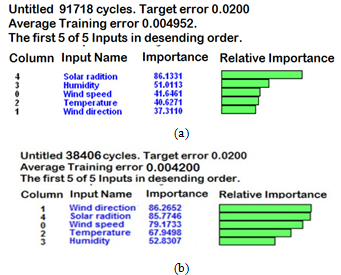
 | Figure 5. Importance of different input on the output (a) PM10 and (b) TSP |
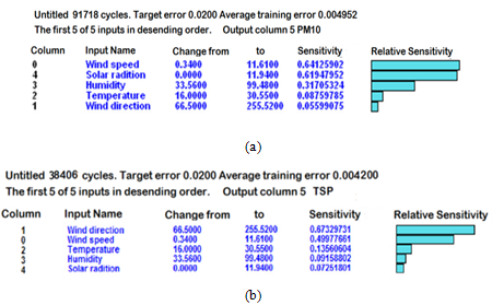
 | Figure 6. Relative sensitivity of different input parameter for (a) PM10 and (b) TSP |
|
3.3. Importance and Sensitivity of Input Parameters on Outputs
- The weights of different input parameters obtained from the network and their relative importance for PM10 and TSP are given in Figure 5 (a, b). The weight represents the importance of input parameter in the network. In the input column, the solar radiation shows the highest importance on PM10 (Figure 5a) and the wind direction on TSP (Figure 5b). Insignificant difference between the weights of wind direction (86.27) and solar radiation (85.77) in the input column of TSP reveals their analogous influence on TSP. Roy and Adhikari (2009) also observed significant role of these parameters on particulates. The order of importance for wind speed and temperature is same for both PM10 and TSP indicating that these parameters have similar influence on particulates.The sensitivity of different input parameters and their relative sensitivity are shown in Figure 6 (a, b). The inputs are shown in the descending order of sensitivity from the most sensitive input. It shows how much an output changes when the inputs are changed. The change in the output is measured as each input is increased from the lowest to the highest. In general, the order of different input parameters for PM10 and TSP is different for importance and sensitivity, but for TSP, the wind direction has similar rank in the input column for importance and sensitivity indicating that it has a significant role in variation of coarser particle concentrations. The wind speed is the highest sensitive for PM10 showing that slight change in wind speed can reveal a major fluctuation in fine particle concentrations.
3.4. Prediction with Training Examples and Performance
- Predictions of output for the training examples show average training error as 0.004952 and 0.004200 for PM10 and TSP respectively (Figure 7). These values below target error indicate performance of the models. The position of the values on both axes is scaled from 0 to 1. Predicted outputs for training examples get closer to the true values as training progresses. If the predicted values are very close to the true values then the dots will be on the diagonal line.
 | Figure 7. Predictions of output for the training examples of (a) PM10 and (b) TSP |
4. Conclusions
- Though target error, learning rate, momentum, number of hidden layers were same for PM10 and TSP but number of cycles, number of hidden neurons and weights in different hidden layer, the order of relative error for different sets of data, importance and sensitivity sequence of imput parameters varied. It was observed that the solar radiation obtained the highest rank of importance for PM10 and the wind direction for TSP. The wind speed and temperature showed similar order of importance for PM10 and TSP indicating their same influence on particulates. From the sensitivity columns, it was found that the wind speed is the highest sensitive on PM10 and the wind direction on TSP indicating that slight variation in these input parameters will have significant fluctuations in particulate concentrations. Percentage difference between predicted and measured values revealed that developed neural networks models can be used for the assessment of particulate concentrations in the study area using meteorological data as input parameters.
ACKNOWLEDGEMENTS
- The author is thankful to the Director, National Institute of Rock Mechanics (NIRM) for in-house funding of this project. He is grateful to Dr. G.R. Adhikari, Scientist & Head, Technical Coordination & Project Management Department, NIRM for his valuable comments.
 Abstract
 Reference
 Full-Text PDF
 Full-Text HTML