1. Introduction

Tomato (Lycopersicum esculentum L.) is widely cultivated across the globe due to its edible fruit [1] and its service as important inputs for food industries [2]. It is of high commercial value because of its high nutritive value [3]. It is composed of several species [4] which performed differently across locations. Therefore, multi-location trials must be carried out to ascertain stability across environments [5].

Mostly, results obtained reflect variations in yield of tomato from one location to another in which the genotype with best performance in one location often shows inconsistency in other locations. This is due to interaction between genotypes and the environment [6]. The environment has a great influence on the expression of quantitative traits and this affects genotypes when grown in different environments. Whenever genotypes grown in different environments differ in their performance across environments, there is Genotype x Environment (G x E) interaction and this can affect response to selection. In a situation when a set of genotypes does not change across environments, it is called non-crossover interaction [7]. Cultivars can bring about good performance when grown under a wide range of environments, thereby giving them broad adaptation, or narrow (specific) adaptation under specific growing conditions [8]. Differences in genetic structure also contribute to G x E interaction (GEI) due to different characteristics of variety type with low heterogeneity or heterozygosity [9].

The most important characteristic of a genotype before it can be released is yield stability [10,11]. Yield stability refers to the ability of a genotype to withstand variability in yield over a wide range of environmental conditions while adaptation is the ability of a genotype to perform well across a wide range of geographical regions with varying climatic conditions [12]. Genotypic adaptation is usually quantified using yield-response. GEI affects the expression of a genotype phenotypically, and this leads to the use of stability analysis to evaluate the performance of the genotypes across varying testing environments for better selection by plant breeders [12].

The two most powerful statistical tools for multi–environment trial (MET) data analysis by researchers are the additive main effects and multiplicative interaction (AMMI) model and the genotype main effect plus genotype × environment interaction (GGE) biplot methodology [5]. [5] further identified the major disadvantage of the AMMI model to be its insensitivity to the most important part of the crossover GEI. Some of the disadvantages of the AMMI model have, however, been taken care of by the GGE biplot methodology. Among other numerous advantages, the GGE biplot methodology is proficient in identifying the best genotype in a particular environment, as well as the most suitable environment for each genotype [5].

The GGE biplot methodology has recently gained popularity because of its ability to analyze an array of data using two-way structure [13]. Similarly, AMMI model has been used of recent due to the fact that it combines the classical additive main effects model for G x E interaction with the multiplicative components into an integral least square analysis which has led to its effectiveness in selection of stable genotypes [14]. It fits the additive main effect of genotypes and environments using analysis of variance and then describes the non-additive parts and the GEI using principal component analysis (PCA) [13]. The utilization of the GGE biplot technique for the analysis of trait and quantitative trait loci interactions in barley was described by [15].

There has been high demand of tomato especially in African due its high nutritive content and daily consumption in human diet. Therefore, crop improvement programme must be on the increase. In any crop improvement programme, performance of the promising genotypes across different growing areas of the crop and climatic conditions must be evaluated. This is to ascertain the genotypes with high yield and stability in performance under different environmental conditions. Hence, it becomes important to use the two tools complementarily in order to achieve the best result in a MET study. The objectives of the study were to evaluate the yield of selected tomato genotypes over successive years and under varying climatic conditions (wet and dry seasons) and to identify tomato genotypes with high stability and adaptability for yield across test environments.

2. Materials and Methods

The experiment was conducted at the Vegetable Research Field of the National Horticultural Research Institute (NIHORT), Ibadan, Nigeria, situated on Latitude 07° 24.204’’N and Longitude 03° 50.895’’E, at an altitude of 178 m above sea level. Twelve tomato genotypes selected based on yield and resistance to Fusarium wilt disease were used for this study. The seeds were drilled into nursery trays filled with steam sterilized top soil and watered at two days interval for four weeks. Compost manure was applied to the field at the rate of 1.4 tons/ha at one week before transplanting to allow decomposition of the compost material and for nutrients to be readily available in the soil for plant use. The experiment was arranged in a randomized complete block design with three replicates during the wet and dry seasons of the year 2016, 2017 and 2018 creating a four year-season environments. A plot size of 2.5 m x 0.6 m and a spacing of 0.5 m x 0.6 m were used. Weeding was carried out at two weeks interval while Cypermethrine insecticide (10% E.C.) was applied at 10-days interval for four consecutive times. Data were collected on plant height, number of leaves per plant, number of branches per plant, number of fruits per plant, fruit weight per plant and unit fruit weight. The pooled data were subjected to analysis of variance while the stability, adaptability and performance of the tomato genotypes across the four year-season environments in derived savannah area of Ibadan, Nigeria were also determined.

These yield data were subjected to AMMI analysis using Statistical Analysis Software (SAS).

The linear model for AMMI, according to [16] is:

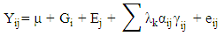• Y_ij = the yield of the i^th genotype in the j^th environment;

• µ = the grand mean;

• G_i and E_j = the deviation of the i^th genotype and the j^th environment from the grand mean respectively;

• λ_k = the square root of the eigen value of the PCA axis k;

• α_ik and γ_jk = the principal component scores of the i^th genotype and the j^th environment, respectively, for PCA axis k;

• e_ij = the error term

GGE Biplot analysis: Singular Value Decomposition (SVD) of the first two principal components were used to fit the GGE biplot model [15].

The linear model of GGE biplot is:

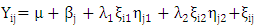• Y_ij is the trait mean for genotype i in environment j;

• μ is the grand mean;

• β_j is the main effect of environment j; μ + β_j being the mean yield across all genotypes in environment j;

• λ₁ and λ₂ are the singular values (SV) for the first and second principal components (PC1 and PC2), respectively;

• ξ_i1 and ξ_i2 are eigenvectors of genotype i for PC1 and PC2, respectively;

• η_j1 and η_j2 are eigenvectors of environment j for PC1 and PC2, respectively;

• ξ_ij is the residual associated with genotype i in environment j [17].

3. Results

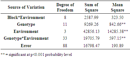
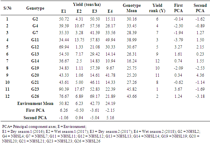
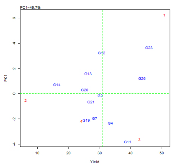
The combined analysis of variance revealed highly significant differences (p ≤ 0.01) for environments, genotypes and genotype by environment interaction indicating differences in performance of genotypes across environments (Table 1). The application of AMMI model in partitioning of G x E indicated that the first two principal component axes scores were statistically significant. The AMMI analysis reported in Table 2 and Fig. 1 showed that the first two principal component axes (PCA 1 and PCA 2) explained 49.7% and 44.5% of the total variation.

Table 1. Combined Analysis of Variance for fruit yield of 12 genotypes grown in four environments

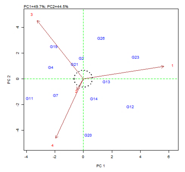Figure 1. Vector-view of the AMMI biplot of fruit yield showing the relationship between genotypes and the test environments

Both axes accounted for 94.2% of the existing diversity. The mean fruit yield of genotypes ranged from 16.24 tons/ha for Genotype 14 (NHSL14) to 45.82 tons/ha for Genotype 23 (NHSL23) while the mean fruit yield of environment ranged from 6.23 tons/ha for Environment 2 to 50.82 tons/ha for Environment 1 (Table 2).

Table 2. Yield for 12 tomato genotypes grown in four environments, their mean values and first PCA scores from AMMI analysis

The Vector-view of the AMMI biplot for fruit yield showing the relationship between genotypes and the test environments is presented in Figure 1 and it revealed that NHSL26 ranked first across the test environments. Genotypes NHSL2, NHSL20 and NHSL21 were the closest to the origin of the biplot, and are, therefore, adjudged to be the most stable among the high yielders. However, genotype NHSL2 had a mean yield of 30.16 tons/ha which is greater than the overall mean yield of genotypes (29.84 tons/ha) while NHSL20 had a mean yield of 25.20 tons/ha and genotype NHSL21 had a mean yield of 27.26 tons/ha, and these values were lower than the overall mean yield of genotypes. This disqualifies genotypes NHSL20 and NHSL21 from being a candidate genotype for selection.

On the other hand, genotypes NHSL11, NHSL12, NHSL23 and NHSL26 with mean yield higher than the overall mean yield of genotypes, and genotype NHSL19 whose mean yield was lower than the overall mean yield were identified as the most unstable genotypes.

Genotypes NHSL4, NHSL7, NHSL13 and NHSL14 present intermediate stability. Of the four test environments, E2 had the shortest vector, and closest to the biplot origin. Also, an acute angle was observed between Environments E2 and E4 (where genotypes NHSL7 and NHSL11 were found), and this showed that they were closely related (judging from the positive correlation ween them). However, obtuse angles were observed between Environments E1 and E4, E1 and E3, and E2 and bet E3, and this showed that they were slightly negatively correlated (according to the rule of the equation: ‘r_ij = cos α_ij’, where r = the correlation coefficient between the i^th and j^th environments, while α_ij = the angle between the vectors of the i^th and j^th environments).

Figure 2 presents the AMMI biplot showing main (genotype and environments average yield) effects and interactions as PC1 scores. Genotypes and environments situated at the right hand of the graph revealed yield levels that were above the overall average. Genotype NHSL23 was the highest yielder and it interacted well with environment E1 while genotype NHSL26 was the second overall best but it did not interact well with E1. Genotypes NHSL4 and NHSL11 are high yielding and adaptable to environment E3 while genotypes NHSL2, NHSL7, NHSL21 and NHSL19 were low yielding but well adapted to environments E2 and E4. Genotypes NHSL12, NHSL13, NHSL14 and NHSL20 did not have any environment and were therefore poor performers across the tests environments.

Figure 2. AMMI biplot showing main (genotype and environments average yields) effects and interaction as PC 1 scores

Figure 3 shows the average-environment axis (AEA) view based on the mean performance and stability of the genotypes. Genotype NHSL26 recorded the highest mean yield, followed by NHSL23, NHSL2, NHSL4 and NHSL19 while NHSL14 had the lowest mean yield, followed by NHSL20. Genotype NHSL11 was found to have a mean yield similar to the overall mean. The GGE biplot showing the discriminating and representativeness view of the test environments was presented in Figure 4. Environment E2 had the smallest acute angle with the AEA, followed by E3, and then E1. Environment E4 had an obtuse angle with the AEA.

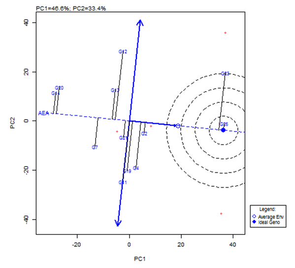Figure 3. The average-environment axis (AEA) view to show the mean performance and stability of the genotypes

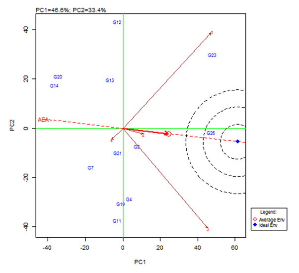Figure 4. GGE Biplot showing the discrimination and representativeness view of the test environments (with Average-Environment-Axis (AEA))

The most discriminating environment is the one that is most informative. This is measured by the concentric circles on the biplot origin which help us to determine how long the environment–vector is, and this length is proportional to the standard deviation found in the respective environments [17]. Therefore, environments E1 and E3 were identified as the most discriminating environments while environments E2 and E4 were the least discriminating (non-informative).

The polygon view (which displays “which-won-where”) of the GGE biplot analysis of 12 tomato genotypes tested in four environments is shown in Figure 5. It displays which genotype performed best in which environment. This polygon is formed by connecting the genotypes that are furthest away from the origin of the biplot in such a way that other genotypes fall within the polygon. From the origin, a perpendicular line was drawn to each side of the polygon in which each line extends out of the polygon, dividing it into five resultant sectors. Whenever environments fall into different sectors, different genotypes won in different sectors while a crossover G x E pattern is in place (Figure 5).

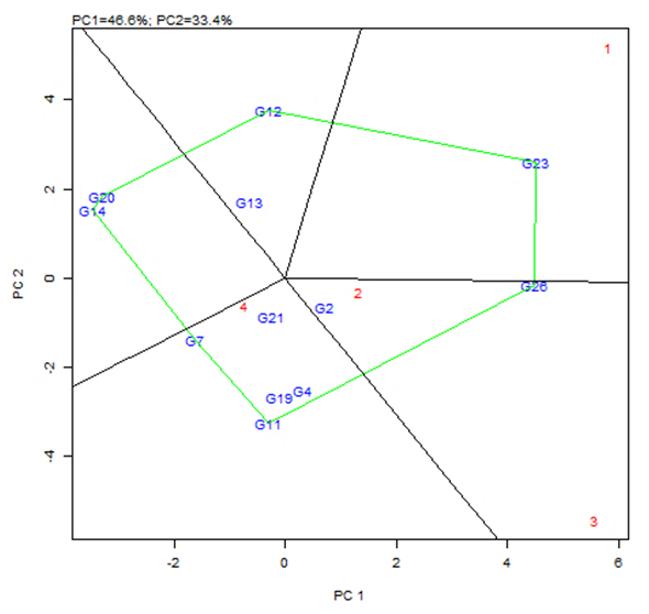Figure 5. The polygon view (which-won-where) of the GGE biplot analysis of 12 tomato genotypes tested in four environments

The winning genotype of any environment or set of environments is therefore the genotype at the vertex of each sector. However, a vertex genotype where no environment exists is considered to be the poorest performer in that test environment. In environment E1, NHSL23 was the winning genotype; NHSL26 was the winner in environments E2 and E3 while NHSL11 was the best performer in environment E4. However, NHSL12 and NHSL14 were vertex genotypes in sectors with no environment and were therefore referred to as poor performers in the test environments. All other genotypes that do not fall on the vertices or close to the vertices were not adaptable to any of the environments. The genotypes that were close to the origin of y-axis were more stable than those far away.

4. Discussion

The objective of most crop breeders is to develop varieties that will perform consistently well across multiple environments. The highly significant differences for environments, genotypes and GEI implied that the four environments significantly influenced the expression of the GEI and the genetic diversity that existed among the genotypes. It also implied that the environments were able to discriminate among the genotypes. Thus, it is possible to make a selection of stable genotypes from among the genotypes used. Similar results have also been obtained in tomato genotypes [18,19], as well as other crops such as rice [16,10], bread wheat [20] and sugarcane [21,22]. The fact that there was a significant GEI effect in the present study indicated that the genotypes evaluated were not consistent in performance across environments and the magnitude of the GEI needs to be determined [23]. This could be the reason why half of the genotypes evaluated had mean values above the overall genotype mean while the remaining half had values below the overall mean. Thus, the GEI was successfully partitioned by using the AMMI model, and this indicated that the first two principal component axes scores were significant and accounted for 94% of the total variation.

Adaptability is the ability of a genotype to perform well across a wide range of geographical regions with varying climatic conditions while yield stability refers to ability of a genotype to withstand variability in yield over a wide range of environmental conditions [24,12]. The IPCA biplot scores are an indication of genotype stability. The greater the IPCA scores, either negative or positive, the more adapted a genotype to a particular environment [25]. The high (though both positive and negative) scores of genotypes such as NHSL23, NHSL11, NHSL12 and NHSL4 explain the reason why they ranked first and second in the test environments, hence their potentials for being selected as high yielding and adaptable genotypes in the test environments. This is congruent with the work of [17]. Furthermore, an overview of the IPCA scores reflects a disproportionate response of the genotypes. Thus, the genotypes are ranked differently in each of the environments [16]. This implies that a crossover type of GEI exists and it is useful for specific adaptation, [24,17].

In the AEA biplot view, the single–arrowed line (AEA abscissa) points to the genotype with the highest mean yield across environments while the double-arrowed line (AEA ordinate) points to greater dissimilarity (or poorer stability) in any of the two directions. According to [26], the higher the projection of a genotype from AEA coordinate axis, the lower the stability of the genotype and the greater the interaction with the environment. An ideal genotype should possess both high mean yield and high stability across the test environments. Hence, genotype NHSL26 was the ideal genotype showing higher yield across all the environments; NHSL2 was the most stable followed by NHSL21 while NHSL12 was the most unstable genotype.

The genotype performance and stability can be seen from the GGE biplot, which is a graphical representation of the association between genotypes and environments [17]. The high percentage of total variation observed for principal component axes, PC 1 and PC 2 indicated that the biplot is suitable and adequate for the approximation of environment-centered data. The fact that genotype NHSL23 had the longest vector indicated that it was most unstable but adaptable to an environment. This suggests that it can be recommended for specific environment and is among the environmentally most responsive genotype. Genotypes NHSL2 and NHSL21 that have vectors closest to the origin of the biplot, making them among the environmentally least responsive and can therefore be used in breeding for wider adaptation or stable performance across environments. However, due to the relatively low mean yield of genotype NHSL21, genotype NHSL 2 is chosen in preference over it. The presence of more than one mega-environment in the study indicates that the four sites differ significantly from one another in terms of discriminating capacity. This is in conformity with the work of [27].

The biplot further shows the discriminating and representativeness view of the test environments and this unveils the similarities among test environments in discriminating the genotypes. This is better achieved with the aid of the line (Average-Environment Axis (AEA)) that passes through the average environment and the biplot origin [17]. The test environment with the smaller angle with AEA is more representative than other test environments. Also, the longer an environment vector is, the more discriminating (informative) it is [28,17]. Thus, in the present study, environment E2 was adjudged the most representative environment because it had the smallest acute angle with the AEA. This implies that it represented the average environment. Similar results were obtained in a study on paddy by [28]. Also, environment E1 was the most informative, providing more information about the genotypes in that environment, and can be used as test environment. Due to the discriminating and non-representativeness of E1 and E3 as test environments, they can be used for selecting specifically adapted genotypes if the target environments can be partitioned into mega-environments.

However, if an environment combines both discriminative and representative together, such can be used as good test environments when selecting for generally adapted genotypes. In this study, there was no environment that combined the two characters. This negates the findings of [17].

The polygon view of the GGE biplot showed that the NHSL23 was the winning genotype in environment 1 (E1), NHSL26 in environment 2 (E2) and 3 (E3) and NHSL11 in environment 4 (E4) while NHSL12 and NHSL14 were the poor performers across the test environments. The NHSL23 gave the best performance in all the test environments.

5. Conclusions

Multi-locational trials are performed to evaluate new or improved genotypes across multiple environments (locations and years) before they are promoted for release and commercialization. This approach helps to increase yield stability and determine the best genotype(s) for an environment. Three genotypes, NHSL23, NHSL26 and NHSL11 produced the highest yields in the four environments. Across the four environments, NHSL23 ranked highest in terms of yield and is considered as best candidate for production while the most stable genotype was NHSL21 and NHSL26 was the most adaptable genotype. NHSL 26 can be considered for areas with moderate to low atmospheric rainfall. These genotypes can be evaluated in more environments to assess their adaptability and possible recommendation for release.