-
Paper Information
- Next Paper
- Previous Paper
- Paper Submission
-
Journal Information
- About This Journal
- Editorial Board
- Current Issue
- Archive
- Author Guidelines
- Contact Us
International Journal of Plant Research
p-ISSN: 2163-2596 e-ISSN: 2163-260X
2012; 2(1): 47-50
doi:10.5923/j.plant.20120201.07
A Predator-Prey Model with General Holling Interactions in Presence of Additional Food
 Abstract
 Reference
 Full-Text PDF
 Full-text HTML
Banshidhar Sahoo
Department of Mathematics, Daharpur A.P.K.B Vidyabhaban, Paschim Medinipur, West Bengal, India
Correspondence to: Banshidhar Sahoo, Department of Mathematics, Daharpur A.P.K.B Vidyabhaban, Paschim Medinipur, West Bengal, India.
| Email: |  |
Copyright © 2012 Scientific & Academic Publishing. All Rights Reserved.
A predator-prey model with general Holling type of interactions in presence of additional food is proposed. The stability of equilibrium points of the system is analysed. The bifurcation analysis is done with respect to Holling parameter as well as quantity of additional food. The model will be useful for construction of real food chain model for predicting future which will be important for bio-conservation and pest management.
Keywords: Predator-Prey, Additional Food, General Holling, Stability
Cite this paper: Banshidhar Sahoo, A Predator-Prey Model with General Holling Interactions in Presence of Additional Food, International Journal of Plant Research, Vol. 2 No. 1, 2012, pp. 47-50. doi: 10.5923/j.plant.20120201.07.
Article Outline
1. Introduction
- Understanding the relationship between predator and prey is a central goal in ecology. One significant component of the predator-prey relationship is the predator’s feeding rate upon prey. The predator’s feeding rate as a function of changes in the density of food items in the habitat is called organism's “functional response”. There are many conceptual food chain models considering specific functional form of predator-prey interaction.Many scholars have studied about continuous food chain models for several functional responses such as Holling-Tanner type[1,2], Beddington-DeAngelis type[3,4] and ratio dependent type[5,6]. But we observe that these functions satisfy some basic biological requirements and have the advantages of mathematical simplicity. However, there is no biological reason to prefer this special type of functional responses, but the exact predator functional response is more important. A realistic interaction function should be based on biological hypotheses. Interaction function should be such that it does not allow the predator to grow arbitrarily fast, even if prey is abundant. Furthermore, the shape of the function for low prey densities can often be guessed. In the intermediate region, between very low and very high prey densities, the interaction function in most cases expected to be increasing [7]. In this sense the Holling functions are not the only realistic interaction functions, but merely the simplest of realistic approximations. Many scholars have studied a food chain model with Holling type-I, type-II or type-III functional responses. The Holling type-II function is based on theassumption that predation rate is proportional to prey density if prey is scarce. If predator actively seeks out large concentrations of prey the Holling type-III are more appropriate. But the functional responses should be of general type[7] for constructing a real food chain model. In fact, in real world, predators of different species may feed on preys in different types of consumption ways. We have now concentrated about two species food chain model with general Holling type of functional responses. The predator-prey model with general Holling interactions is of the form:
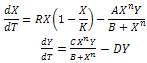 | (1) |
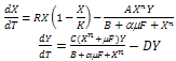 | (2) |
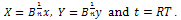 The system (2) reduces to the following form
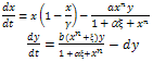 | (3) |
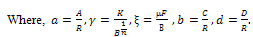 Here “” and “” are noted as control parameters which characterize the “quantity” of additional food available to the predator and its “quality” relative to the prey respectively. The system (3) is to be analysed for x(t)0, y(t)0. In this paper, we first analyse stability criteria of the system (3) theoretically in section 2. The numerical study is done with respect general Holling parameter and quantity of additional food. Finally conclusion is given in section 4.
2. Theoretical Study
2.1. Dissipativeness
- Obviously, the right-hand sides of the system (3) are continuous and have continuous partial derivatives on the state space
 In fact, they are Lipschitzian on
  and then the solution of the system (3) with non-negative initial condition exists and is unique. As the solution of the system (3) initiating in the non-negative quadrant it is bounded, using [9] it is easy to see that
  is an invariant domain of the system (3). Theorem 2.1. The system (3) is dissipative.Proof: From the first equation of the system (3), it easy
  By comparison theorem, we have
  for all
  ,
,  This implies that x(t)≤ γ, for sufficiently large t.Considering (x(t), y(t)) be any solution of the system (3) with positive initial condition, we define
 That is
  .Thus
.Thus  , where
  Applying the theory of differential inequality, we obtain
 For
For  , we have
  .Hence all solutions of the system (3) that initiated in
  are confined in the region
 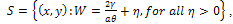 , which means that all species are uniformly bounded for any initial value in
2.2. Stability Analysis
- The system (3) possesses the following steady states:i) The trivial state
 The variational matrix VE0 at E0 is given byii) The axial state
  The variational matrix VE1 at E1 is given bywhich has one eigen value -1 and other is
  The equilibrium point E1 is said to be unstable if
 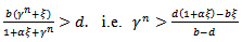 for b>d and
  which is the existence criteria of interior equilibrium point.iii) The interior equilibrium point
  ,where
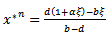
 The existence criteria of E* reveals that
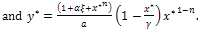
  and y* exists provided
  , from theorem 2.1.Now, we study the stability criteria around E*. The variational matrix of
  is given byWhere
 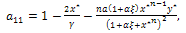 The characteristic equation of
  is where
 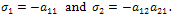 The eigen values are
 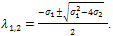 .Here
.Here  then both
 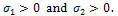 Therefore, two eigen values are negative. Thus the system may be locally asymptotically stable around
  otherwise it is unstable. Thus depending upon system parameters; the system may exhibit stable or unstable behaviour in this case.
3. Numerical Results
- In this section, we have done bifurcation analysis of the system (3) with a set of hypothetical ecosystem parameters, most of which are taken from Srinivasu et al.[8]. The parameter values are taken as γ = 6.0, β = 0.3, d = 0.2, which are remain unchanged throughout simulations. We have done bifurcation analysis with respect to Holling parameter
 as well as quantity of additional food
  .
.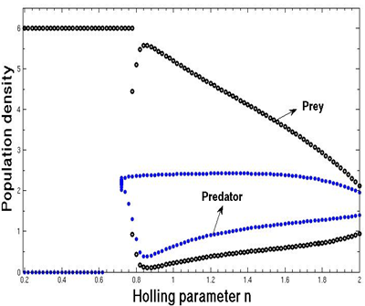 | Figure 1. The bifurcation diagram of the system (3) with respect to Holling parameter n without supply of additional food |
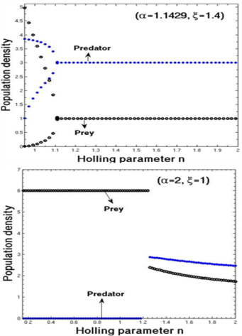 | Figure 2. The bifurcation diagram of the system (3) with respect to Holling parameter n in presence of additional food to predator |
 for
for  without supplying any additional food. From the figure 1, we observe that the prey species has stable dynamics where the predator species extinct for
  Within
  , both prey and predator species have limit cycle oscillations. On the other hand, figure 2 is the bifurcation diagram of the system (3) with respect to Holling parameter
  in presence of additional food to predator. The figure 2 shows that both prey and predator species have limit cycle oscillation within
  and both settles down to steady state for
  in presence of additional food
  Again from the figure 2, we observe that prey species have steady state while the predator species extinct from the system for
  in presence of additional food
  , and both the species have stable dynamics for
  Figure 3 is the bifurcation diagram of the system (3) with respect to quantity of additional food
  to the predator for different values of n and
  . The figure 3 indicates that the system have either limit cycle or steady state in ranges of
  From figure 3, it is important to note that there are no eradication effects in the system in presence of additional food for different functional responses. Therefore, survival of the species in a system depends on interaction functions as well as supply of additional food.
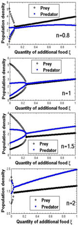 | Figure 3. The bifurcation diagram of the system (3) with respect to quantity of additional food ξ for different values of Holling parameter |
4. Conclusions
- We have formulated a predator-prey model with general Holling interactions in presence of additional food to predator. We have discussed the dissipativeness of the system under certain conditions. The stability criteria of all equilibrium points of the system are derived. The numerical simulation is also shown here. We have seen that the dynamics of the system (3) highly depends on Holling parameter. There is extinction possibility for small values of Holling parameter without supply of additional food. Srinivasu et al. [8] defined that the supply of additional food should be high quality if
 and low-quality if
  Here, in figure 3, we have shown that there is no extinction possibility in presence of high quality of additional food
 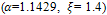 but for low-quality of additional food
  the system has extinction risk for
  . Therefore, the existence of species in a system depends on interaction functions as well as quality of additional food. Here, we have shown that the model with Holling type-II or type-III is not always realistic. Because the model with Holling type-II or type-III is a particular case of general Holling interaction and this assumption is made for only simplicity of the model construction. There is no reason for construction of such special type of interaction function. Therefore, we suggest that choice of interaction function is a very important part of realistic model for prediction of future determining biological strategy. Our study will be useful for construction of a real biological model and pest control.