-
Paper Information
- Next Paper
- Previous Paper
- Paper Submission
-
Journal Information
- About This Journal
- Editorial Board
- Current Issue
- Archive
- Author Guidelines
- Contact Us
Public Health Research
p-ISSN: 2167-7263 e-ISSN: 2167-7247
2012; 2(3): 43-48
doi: 10.5923/j.phr.20120203.02
Time Course of Apparent Temperature Effects on Cardiovascular Mortality: A Comparative Study of Beijing, China and Brisbane, Australia
 Abstract
 Reference
 Full-Text PDF
 Full-Text HTML
Jing Sun1, 2, Guo Xing Li2, Rohan Jayasinghe3, Ross Sadler1, Glen Shaw1, Xiao Chuan Pan1, 2
1School of Public Health and Griffith Health Institute, Griffith University, Q4222, Parkland Campus, Parkland, Gold Coast, Australia
2School of Public Health, Peking University, China, 100191, Beijing, China
3School of Medicine, Griffith University and Cardiac Services/Cardiology, Gold Coast Health District Gold Coast Hospital, Q4222, Parkland Campus, Australia
Correspondence to: Guo Xing Li, Jing Sun, School of Public Health, Peking University, China, 100191, Beijing, China.
| Email: |  |
Copyright © 2012 Scientific & Academic Publishing. All Rights Reserved.
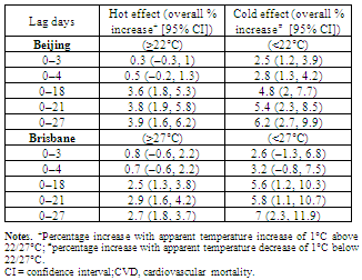
This comparative study aimed to clarify the different characteristics of time course of apparent temperature and their effect on cardiovascular mortality in Beijing, China, and Brisbane, Australia. The present study used polynomial distributed lag models to explore the lagged effects of apparent temperature on daily cardiovascular mortality up to 27 days in Beijing, China (2005–2009), and Brisbane, Australia (2004–2007). The results show a longer lagged effect on cold days and a shorter lagged effect on hot days. The cut-off points in Beijing and Brisbane were 22℃ and 27℃, respectively. In Beijing, a statistically significant association was observed for lags of 0–3 days and lags of 3–18 days on hot and cold days, respectively. In Brisbane, a significant association was found for lags of 3–4 days and lags of 10–21 days on hot and cold days, respectively. The lagged effects extended longer for cold apparent temperature but were immediate for hot apparent temperature. Though the cut-off point in Brisbane was higher than in Beijing, the population in Beijing was more resistant to high temperature above the cut-off point than the population in Brisbane.
Keywords: Temperature, Apparent Temperature, Cardiovascular Mortality
Article Outline
1. Introduction
- Global warming has attracted attention worldwide. According to the Intergovernmental Panel on Climate Change, it is likely that the global average surface temperature will have increased by 1.8–4.0℃ by 2100 (1). Many epidemiological studies have shown that extreme temperature has adverse effects on non-accidental and cardiopulmonary mortalities. In an analysis of data, Le Tertre et al. found that the all-cause mortality in nine French cities increased by 3096 extra deaths in the 2003 heatwave(2). Baccini et al. found that the estimated overall change in all natural mortality associated with a 1℃ increase in maximum apparent temperature (AT) above the city-specific threshold was 3.12% in the Mediterranean region(3). This is consistent with reports from other countries(4-6). Temperature effects are more pronounced in the elderly, women and those with chronic diseases (6-10).Numerous epidemiologic studies have shown that there are lagged effects of temperature on mortality(11, 12). Goodman et al. found that, in the city of Dublin, from 1980 to1996, only considering the acute effects of temperature might underestimate the total effects of temperature on mortality(11). Pattenden et al. reported that, in London, cold effects appeared after lag 3 days and lasted at least 2 weeks(12). However, the impact of temperature on mortality might be affected by the adaptation methods used in different geographical areas (for example, the use of an air conditioner). Few studies are available that compare two cities on different continents and that have different climates. A better understanding of the differences between two cities might be helpful for the development of public health policy. To explore the presence of lagged effects, the time dimension of the relationship between temperature and mortality should be addressed. There are several methods that can be used to study the delayed effects of temperature. Using the moving average of the temperature up to a certain lag is a relatively simple model. However, the limitation of this model is that it cannot show the temporal structure of the temperature effects. The distributed lag non-linear model (DLNM) is an approach based on distributed lag models (13, 14). This model can flexibly show the detailed temporal structure of temperature–mortality relationships for lags and can adequately model the main effects of temperature(13,14).In addition, almost all population studies to date have used mean temperature as meteorological parameter in the analysis of time course of temperaturetemperature. However, it is possible that AT is more appropriate for analysis. AT is an index intended to reflect the physiological experience of combined exposure to humidity and temperature and is thereby better able to capture the effects on health than temperature alone(15, 16).This study explored the lagged effects of AT on cardiovascular diseases in Beijing, China, and Brisbane, Australia, which have typical temperate and subtropical climates, respectively.
2. Materials and methods
2.1. Study Area
- Beijing is the capital of China, located at latitude 39.55′ north, longitude 116.25′ east(See details: http://www. infoplease.com/ipa/ A0001769. html). It is on the North China Plain surrounded by mountains with altitudes of 1000–1500 metres to the west, north and north-east and by the Bohai Sea on the south-east. Beijing has a typical warm temperate semi-humid continental monsoon climate, with hot humid summers and cold dry winters. Our study area included the eight urban areas of Beijing, comprising an area of about 1368 km2, which consist of eight districts with a population of approximately seven million. Brisbane is the capital of Queensland, Australia, located at latitude 27.29′ north, longitude 153.8′ east. Brisbane features a typical subtropical climate, with warm humid summers and mild clear winters. The study area has a population of 0.97 million.
2.2. Mortality and Environmental Data
- In this study, we used data from Beijing, China, and Brisbane, Australia. Daily counts of cardiovascular deaths (I00-I99; International Classification of Diseases, 10th Revision) for the two cities were obtained from the Queensland Health in Australia and the Chinese Center for Disease Control and Prevention in China. The time-series of daily death data available for analysis in each city covered different time periods: for Beijing, data for the five years from 1 January 2005 to 31 December 2009 were available for analysis, while, for Brisbane, data available for the four years from 1 January 2004 to 31 November 2007 were available. The temperature data in Brisbane were collected from the Bureau of Meteorology and, in Beijing, from the National Meteorological Information Center (CMA) of China. Daily air pollution data in Brisbane and Beijing were from the Environmental Protection Agency Australia and the Beijing Municipal Environmental Monitoring Center, respectively. In this study, we used AT, which combines temperature and relative humidity, and is an index of human discomfort. AT was calculated using the following formula:
 ,where ‘Ta’ is air temperature and ‘Td’ is dew point temperature.
2.3. Statistical Analysis
- First, we used an independent model to explore the patterns of the relationship between the temperature and mortality. The independent model is described below.Model 1
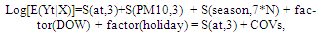 where ‘t’ refers to the day of the observation, ‘E(Yt|X)’ denotes the estimated daily case counts on day t, and ‘S()’ denotes the penalised smoothing spline. ‘PM10’ and ‘at’ represent the current day’s particulate matter with aerodynamic diameter of 10 µm (PM10) concentration and AT, respectively(16, 17). Seven degrees of freedom per year for time were selected so that little information from time scales longer than two months was included(18). This choice largely reduced confounding from seasonal factors and from longer-term trends. ‘N’ denotes the number of years, while ‘DOW’ represents the day of the week. ‘Holiday’ was treated as a dummy variable (0 or 1 denote ‘not a holiday’ or ‘a holiday’, respectively)(19).There were J- and U-shaped associations between temperature and mortality as shown in figure 1 for Beijing and Brisbane, respectively. In Beijing, the J shape pattern suggests that there is no sharp increase in mortality with the increasing apparent temperature. However, in Brisbane, the U shape indicates there is a clear and sharp increase in mortality with the increasing apparent temperature. Temperature stratification cut-offs were determined by Akaike’s Information Criterion(AIC) values.AIC values were calculated using 1℃ increments in mean temperature from 15 to 30℃. The apparent temperature range was selected based on visual inspection of the plots(20-22). The temperature corresponding to the model with the lowest AIC value was chosen as the threshold temperature. We used threshold models as follows.Model 2
 where ‘Th’ and ‘Tc’ are the hot and cold thresholds; the same covariates as in Model 1 were adjusted.A DLNM was used to analyse the lagged effects of mean temperature on CVD for Brisbane and Beijing. To capture the lagged temperature effect, we placed spline knots at equal intervals in the log scale of lags up to 27 days and 4 degrees of freedom for lag according to a previous study(23). We used a DLNM as follows.Model 3
 where ‘TC(TH)’ is a matrix obtained by using the DLNM model below the cold threshold and above the hot threshold; the same covariates as in Model 1 were adjusted.The estimated effects were expressed as the increased percentage of the daily death counts with 1 per increment in the daily AT. All analyses were performed using R software, version 2.11.1 (R Foundation for Statistical Computing, http://cran.r-project.org/), using the Multiple Smoothing Parameter Estimation (MGCV) and Distributed lag non- linear models (DLNM) in R.
3. Results
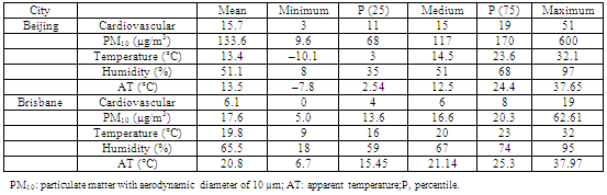
- Table 1 provides summary statistics for the two cities during all seasons. The mean number of deaths from cardiovascular mortality was 15.7 and 6.1 for Beijing and Brisbane, respectively. The corresponding ambient PM10 concentrations were 133.6 g/m3 and 17.6 g/m3, respectively. The mean temperatures were 13.4℃ and 19.9℃ for Beijing and Brisbane, respectively. The ATs in Beijing and Brisbane were 13.5℃ and 20.8℃, respectively.Figure 1 shows the non-linear relationship between mean temperature and mortality in the two cities. It is evident that the pattern of the association between AT and mortality exhibits a J shape for Beijing and a U shape for Brisbane. Based on these results, a threshold model was used to explore the lagged effect of cold and hot temperature. According to AIC, 22℃ and 27℃ were chosen as the cut-off points in Beijing and Brisbane, respectively.Figure 2 shows the three-dimensional plots between AT and mortality at all lag days. It is obvious that the lagged effects in the cold temperature range were of longer duration than those in the high temperature range in both cities. In Brisbane, cold effects lasted for more lagged days than in Beijing.
|
 | Figure 1. Dose-response relationship between apparent temperature and mortality in Beijing and Brisbane. AT: apparent temperature; RR: relative risk |
 | Figure 2. 3-dimensional plots between apparent temperature and mortality at all lag day. RR: relative risk; AT: apparent temperature |
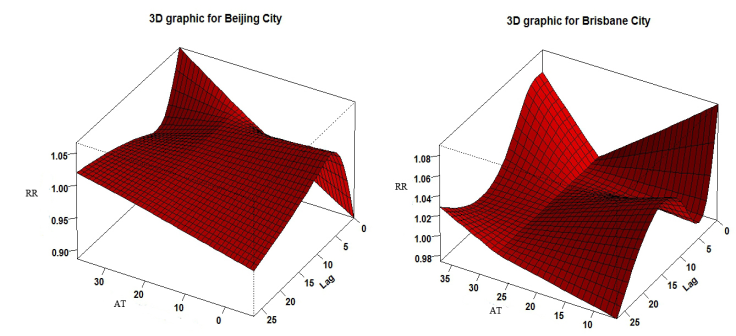
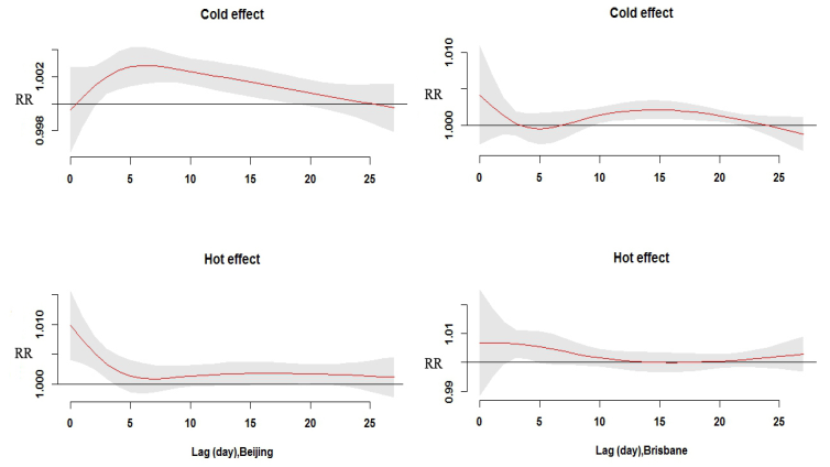 | Figure 3. Relative risks of cardiovascular death (CVD) with an increase (or decrease) of 1℃ in apparent temperature up to 27 days in Beijing and Brisbane. RR: relative risk |
|
4. Discussion
- To our knowledge, this is the first study to quantify the lagged effects of AT on CVD in two cities with temperate and subtropical climates, respectively, in different hemispheres. This study may provide useful knowledge about the different characteristics of climate and adaptation patterns in Brisbane and Beijing and their effects on CVD. In this study, the lagged effects up to 27 days on CVD for both cold and hot AT were examined. A delayed effect of approximately three weeks was observed for cold; however, hot effects were relatively shorter, within one week. In this study, we found an effect of latitude on CVD: cities at higher latitude had lower threshold temperature. Beijing had a relatively lower threshold temperature compared with Brisbane. This finding is similar to that of Chung et al.’s study, which found that Seoul had a relatively higher threshold temperature compared with Beijing with regard to cardiovascular mortality(20). We also found that mean AT in Brisbane is higher than that in Beijing, which might partly explain the different threshold AT. In 13 Spanish cities, Iniguez et al. also found that minimum mortality temperature rose as the mean temperature of the cities increased(24).It is biologically plausible that temperatures can affect health outcomes. First, high temperatures may increase cardiovascular mortality. Nayha reported that high temperature dilates skin vessels and facilitates sweating, leading to a decrease in blood pressure, loss of fluid and salt, and the risk of thrombosis(25). Basu and Samet(26) and Bouchama and Knochel(27) found that high temperature increases heat loss through increased skin-surface blood circulation, which may be related to increased mortality. Second, cold temperatures may also increase the risks of cardiovascular mortality. Keatinge et al. reported that exposure to cold can increase plasma viscosity and arterial pressure in the first hour, contributing to coronary and cerebral thrombosis(28). Cold temperature can also increase plasma cholesterol and plasma fibrinogen, which can lead to thrombosis and acute cardiac events(26,27). Third, a population may be sensitive to different types of CVD in high/low temperatures. Hong et al. used a case-control design to analyse the risk of ischemic stroke during cold temperature days in Incheon, Korea, from 1998 to 2000. They found that cold temperature can increase stroke occurrence(29). Nayha reported that coronary heart disease increased steeply on hot temperature days(25). Braga et al. found that for myocardial infarctions, the effect of heat was larger than the effect of cold(30).In this study, the strongest effects of heat were found immediately after exposure in both cities. Braga et al. found that the lagged effect of hot days was no more than seven days in US cities(30). Gasparrini et al. also found that the lagged effect of hot temperature was immediate for mortality(17). However, cold-related mortality was found to persist for approximately three weeks in both cities in our study. Carder et al. found that in the low temperature range, the cold effect tends to remain at lag periods greater than 14 days(31). Other researchers also reported similar results (32, 33). We also found that the relationship between AT and mortality was different in the two cities as shown in J and U shape in Figure 1. One possible explanation for our finding is that the two cities have different climate characteristics, living conditions and lifestyles as well as different medical insurance systems, which can modify the effect of temperature on mortality. For example, the range of AT is 45℃ in Beijing, well above 31℃ in Brisbane. Another explanation is that human adaptation to climate change is different. A population in a subtropical area might be more resistant to high temperature than a population in a temperate area. Many epidemiological studies have provided convincing evidence that air pollution can increase the risks of CVD in different parts of the world. Schins et al., for example, observed that ambient particles increased tumour necrosis factor alpha and glutathione depletion in a rat study(34). Wu et al. and Fang et al. found that ambient particulate matter could increase the risk of heart disease(35, 36). Therefore, in this study, we assessed the association between AT and mortality after adjustment for air pollutants in the models.This study has several strengths. First, to our knowledge, this is the first research on the extended characteristics of AT on CVD in cities in China or Australia. Second, the index of AT combines temperature and humidity together, which may better reflect the human experience of these. Third, the DLNM was employed to avoid the collinearity of the ATs on days close together. Our study also has several limitations. First, the data on meteorological factors and PM10 used in this research were the average levels in the two cities; hence, a degree of bias from measurement errors may be possible. Second, the density and population characteristics varied in the two cities. There might also be some important confounders, such as ozone, as suggested by Schwartz et al., who found that ozone was associated with mortality(37).In this study, we found different lagged characteristics of cold and hot AT. Cold effects lasted longer than hot, which could provide guidance for policy making. Different targeted efforts in different climate type areas should be used in preventing the adverse effects of climate change. For example, prevention method should be taken in Beijing when AT is progressively lower than or higher than 22℃; and in Brisbane when AT is progressively lower or higher than 27℃.
5. Conclusions
- This study found that the lagged effects of low AT on CVD had a longer duration than those of high AT. The susceptibility to temperature in different areas was different. Population at low altitude was more resistant to high temperature. Further studies are still needed to generalise our findings.We found different patterns in relation to the effect of particular matter and temperature on population mortality in Beijing and Brisbane. In Brisbane, the results indicate a significant increasing mortality rate with increasing temperature and PM10 concentration. The increasing mortality in Beijing shows a different pattern when temperature and PM10 concentration increased. It is noted that the PM10 concentration in Beijing is ten times higher than in Brisbane and the temperature range in Beijing (–10 to 35℃) is much wider than that of Brisbane (10–35℃). However, people in Brisbane were more sensitive to the increasing temperature and PM10 concentration than people in Beijing, as indicated by the increasing mortality rate in Brisbane.
ACKNOWLEDGEMENTS
- We thank the Chinese Center for Disease Control and Prevention. This project was supported by the National Natural Science Foundation of China, grant no. 30972433; Peking University Health Science Center Fund, BMU20110244.