Sikiru A. Ahmed1, Nelson O. Obi-Egbedi2, Idowu Iweibo2
1Department of Chemistry, University of Agriculture, Abeokuta, Nigeria
2Department of Chemistry, University of Ibadan, Ibadan, Nigeria
Correspondence to: Sikiru A. Ahmed, Department of Chemistry, University of Agriculture, Abeokuta, Nigeria.
| Email: |  |
Copyright © 2012 Scientific & Academic Publishing. All Rights Reserved.
Abstract
In this paper, we present a general expression originating from quantum-mechanical perturbation treatment of electronic intensities and Hamiltonian operators for the system (HA and HB) of an absorber and a perturber respectively. The expression is related to the Longuet-Higgins’ definition of solute-solvent interaction and fitted into linear regression mode for the determination of transition polarizabilities of 9H-xanthene, 9H-xathone and 9H-xanthione. The result conforms to those earlier obtained when all possible interaction modes are considered.
Keywords:
Quantum-Mechanical, Hamiltonian Operator, Solute-Solvent Interaction, Linear Regression Mode, Transition Polarizabilities
Cite this paper: Sikiru A. Ahmed, Nelson O. Obi-Egbedi, Idowu Iweibo, Solvent Perturbation of the Electronic Intensity of Solvated Absorbing Molecules, Physical Chemistry, Vol. 2 No. 1, 2012, pp. 16-20. doi: 10.5923/j.pc.20120201.04.
1. Introduction
Various authors have studied the solvent perturbation effects on the electronic intensity of a system consisting absorbing solute molecules. For instance, Weigang[1] applied a second order quantum-mechanical perturbation theory to develop a quanta theory based on the assumption of a spherical cavity, Lorentz field modification of the photon field and the Onsager reaction field for the solute. A similar work by Liptay[2] utilized the modified Onsager-Böttcher reaction field in his formulation. Robinson[3] formulated a theory for a single perturber at a fixed inter-nuclear distance with the solute and presented the mechanism by which the forbidden electronic intensity is enhanced by solvent perturbation. Bayliss and Will-Johnson[4] adapted Linder’s[5] treatment of dispersion interaction between the solute and solvent by a rapidly oscillating electric field to formulate ‘‘field simulation model’’.Linder and Abdulnur[6], in their formalism applied quantum-statistical perturbation method to account for the translational fluctuations in fluid. Abe[7] applied Onsager cavity field model to derive expression which relates the oscillator strength in solution to that in vapour phase. Myer and Birge[8] utilized quantum-mechanical perturbation method to derive the expression that relates the oscillator intensity to the transition moment of an unperturbed cylindrical solute.In this paper, rigorous and general expression that accom modates solvent perturbation of electronic intensity parameters such as stark terms, Einstein coefficient, transition moment, oscillator strength etc was derived and employed in the linear regression mode for the determination of molecular transition polarizability.
2. Objectives
The objectives are to:i. Derive expression from the perturbation of electronic intensities as an alternative to those derived from the perturbation of transition energies.ii. Applying the derived equation for the determination of transition polarizabilities of some molecules.Use modified Onsager-Abe-Iweibo reaction field model to calculate the oscillator strength, f, in vapour phase
3. Methods
Experimental9H-xanthene, 9H-xanthone and 9H-xanthione, n-hexane, cyclohexane are the products of Tokyo Kasei (Japan), and are of spectroscopic grade. Methanol, ethanol, n-butanol, dichloromethane, chloroform, 1, 4-dioxane, acetonitrile, tetrachloromethane were obtained from the British Drug House Ltd and were distilled several times.Electronic absorption spectra were measured at room temperature using Schimadzu UV-1650 double beam spectrophotometer coupled with UV-probe® 2.31 version, operated in the wavelength region 190-500nm. Stock solutions of each compounds dissolved in different solvents were prepared in 5ml standard flasks and are in the concentration range 10-5-10-6M. The quartz cells used were of 1.0cm in optical path. The other experimental conditions are has been described previously by Iweibo et al[9].Theoretical DerivationConsider an ensemble of molecules of two types; type A being the solute or absorber and type B the solvent or perturber. The Hamiltonian operator for the system (A, B) is described by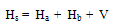 | (1) |
where Ha is a function of electronic and nuclear coordinates of A and Hb those of molecules B, V is the energy operator and a function of molecule A and B, and the distance between them. The distance between A and B assumed to be a weak one and the distance apart of A and B is such that no electron exchange can occur between the solute and solvent. The zero-order wave function of the system can then be adequately described by the orthogonal set of product wave functions, αiBk, which are solutions of the pertinent Schrodinger equation. The effect of solute-solvent interaction, V, is that the zero-order wave function, described by αiβk, is modified by the perturbation to the form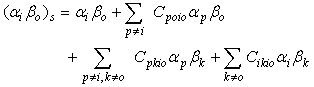 | (2) |
Equation (2) depicts the case of the excited state wave function, in which α refers to the solute and β to the solvent. The ground state equivalent of the wave function in Equation (2) is obtained by replacing i and o in the expression for the excited state wave function.Assuming that the dipole moments operator is given by  | (3) |
where μa and μb are the dipole moments of the solute and solvent respectively, then the complete transition moment is given by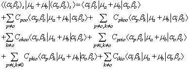 | (4) |
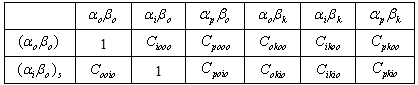
In Equation (4), the higher order terms containing C2 and CC have been neglected on the premise that such terms contribute virtually little or nothing to the C terms because the denominator of each C term is much larger than its numerator.Analysis of each term on the right-hand side of Equation (4) indicates that many terms or components of terms vanish by virtue of the orthogonality of the wave functions in the overlap integrals that multiply such terms and by virtue of the cancellation due to the addition of terms such as C00i0μboo and Ci000μboo as shown in table 1. Under this condition Equation (4) reduces to Equation (5).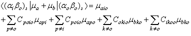 | (5) |
Table 1. Multiplicative table of mixing coefficients of C terms
 |
| |
|
In equation (5), the notation has been simplified such that  which is the transition moment of the solute from ground state
  to the excited
  .Introducing Longuet-Higgins’[10] rigorous definition of the electrostatic interaction energy given as
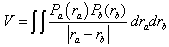 | (6) |
where Pa(ra) is the charge density at the point ra and Pb(rb) that at the point rb. In order to expand each C perturbation term in Equation (5) and solve them in terms of molecular properties, V is approximated to  . This, for example, permits the solution of the term
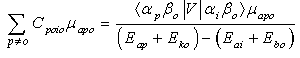 | (7) |
 | (8) |
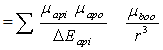
where rab is the sum of the ratio of the solute molecule and that of the solvent molecule. Further analysis is simplified by pairing such solved terms, namely; terms two and three on one hand and terms four and five on the other hand in Equation (5) to give 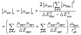 | (9) |
Dividing and multiplying the second term on the right hand side of equation (10) with 3/2 and with  respectively, equation (9) becomes
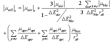 | (10) |
 is the transition moment of the solute and
  is the transition moment of the solvent,
  is the transition energy or ionization potential of the solute and
  is the corresponding one for the solvent molecule. Δα- the transition polarizability is defined by the term in the circular brackets in Equation (9) and (10).Using Labhart[11], and Donath[12] formalism, Equation (10) can be transformed into Equation (11) by equating
  to
to  i.e.
i.e.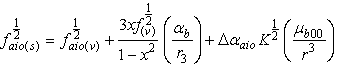 | (11) |
where  and
and  are the root of the oscillator strength in vapour phase and solution respectively.
 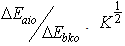 is the root of Einstein coefficient.For the purpose of this study, Equation (11) is rearranged into the following convenient linear regression forms.
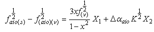 | (12) |
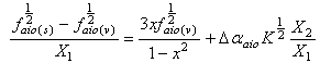 | (13) |
The dependent variables are  and
and in Equations (12 and 13), respectively; and the independent variables are X1, X2 in equation (12) and
  in equation (13). These two equations satisfy the statistical criterion for regression or graphical analysis and the slopes give the values of Δα. In the present study, solvent parameters such as molar refraction and polarizability were fitted into the model using Clausius-Mossotti’s expression[13]. The electronic intensities as defined by oscillator strength and Einstein coefficient in solution and vapour phase were determined using the modified Onsager-Abe-Iweibo reaction field model[14] and the expression that relate oscillator strengths in solution to those in vapour phase was adopted as presented by Abe and Iweibo[15]. The molecular data for the generation of
  X1, X2 and
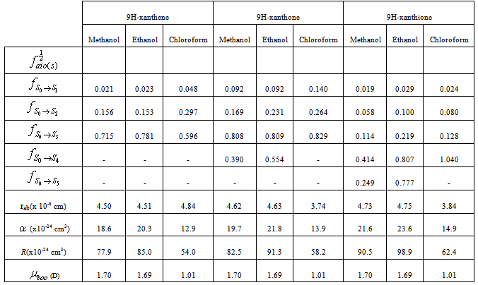
  for graphical analysis is shown in table 2Figure 1 represents the graphical details of representative plots of 9H-xanthene, 9H-xanthone and 9H-xanthione in various solvents according to equation 13. It is obvious that by setting
  in equation 11 (the condition applicable to studies in non-polar solvent), the transition polarizability of an electronic transition can in principle be determined in non-polar solvent alone. In practice, however, as can be seen in table 2, the range of data covered by the independent variables (X2 and
  ) in non polar solvent is so small that large uncertainties attend such determinations. Although, a much larger range is spanned by the independent variables if polar solvents are used, it can be seen in table 2 that additional data in non polar solvents may still be needed for a reliable determination by regression and graphical analysis.
4. Results
Table 2. Oscillator strengths in solution, Molar refraction, polarizability, solvent dipole moment and approximate molecular radii of 9H-xanthene, 9H-xanthone and 9H-xanthione
 |
| |
|
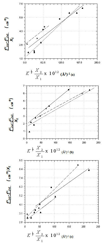 | Figure 1. Plots of data on intensity perturbation of the transitions of 9H- xanthene  , 9H-xanthone , 9H-xanthone  and 9H-xanthione and 9H-xanthione  in (a) ethanol (▪) (b) Chloroform (*) (c) methanol (▲) in (a) ethanol (▪) (b) Chloroform (*) (c) methanol (▲) |
5. Discussion
Oscillator strength of the electronic transitionsFrom table 2, the intensities of electronic transitions in the compounds follow the expected pattern: for example, in 9H-xanthene 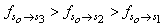 was observed, whereas in 9H-xanthone and 9H-xanthione, it was
 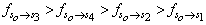 and
and 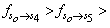
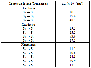
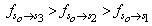 respectively. This implies that the higher the value of f, the more allowed the transition.From table 3, the transition polarizabilities for the three absorption bands observed in 9H-xanthene follow the trend:
 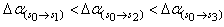 , the trend for the four bands observed in 9H-xanthone is
  , and the trend observed in 9H-xanthione with five absorption bands is
  .The transition polarizabilities increases with energy of the state, the trends above is in line with the submission of Hirschfelder et al, [16] and Chongwain and Iweibo[17] and is supported by the approximate theory which relate the polarizability
  of any state ij to the transition frequency
  between the state i and j, and the oscillator strength
  by
by  where e and
  denote the electronic charge and mass respectively, and
  =2πυij denoting the circular frequency. These trends are reflective of the oscillator strength values for these transitions, and also confirms the positive correlation between the transition polarizabilities (Δα) and the integral Einstein coefficient B.
Table 3. Summary of values for transition polarizability for the observed bands
 |
| |
|
Besides, in line with the free electron molecular orbital (FEMO) theory, the polarizability is proportional to the molecular volume (i.e. Δα α a3, where ‘a’ denotes molecular radii). Consequently, compounds with larger molecular radii show greater transition polarizability. For instance, the molecular radii increase from xanthene to xanthone and to xanthione, so do the transition polarizability. The present analysis agrees favourably with those Abe and Iweibo[18] and reconfirms the earlier result of Abe et al, [19] but disagrees with that of Morales[20]. This marked difference probably arises because Morales considered only the dispersion forces in deriving his expression while the present study takes into consideration all possible interaction modes.
6. Conclusions
The transition polarizabilities determined for the compounds in this paper are being determined for the first time, it is expected that the results obtained will form a database or used for comparison with the results of future determination by electro-optical or other methods.Originating from quantum-mechanical perturbation of electronic intensity, the derived expression in this paper gave low values of oscillator strength in vapour phase compared to those in solution and this reinforces the phenomenon of intensity enhancement of absorbing molecules by solvents.
References
| [1] | O. E. Weigang, Journal of Chemical Physics, 41(5), 1435-1441(1964). |
| [2] | W. Liptays, Zeitschrift fur Naturforschung, 219, 1605-1618 (1966). |
| [3] | G.W. Robinson, Journal of Chemical Physics. 46, 572 (1967). |
| [4] | N. S.Bayliss and G.Wills-Johnson, Spectrochimica Acta, 24A, 551-563(1968). |
| [5] | B .Linder, Journal of Chemical Physics. 33, 668 (1960). |
| [6] | B.Linder and S. Abdulnur, Journal of Chemical Physics, 54 (4), 1807-1814 (1971). |
| [7] | T. Abe, Bulletin of the Chemical Society of Japan, 43, 625-628 (1970). |
| [8] | A. B. Myers and R. R. Birge, Journal of Chemical Physics, 73, 5314- 5314 (1980). |
| [9] | I. Iweibo, P.T. Chongwain, N.O. Obi-Egbedi, and A. F. Lesi, Spectrochimica Acta 47A (6), 705-712 (1991). |
| [10] | H.C.Longuet-Higgins, Proceedings of the Royal Society of London, series A, mathematical and physical sciences. 235, 537-543(1956). |
| [11] | H. Labhart, Helvetica Chimica Acta . 44, 447-449 (1961). |
| [12] | W.E. Donath, Journal of Chemical Physics 39 (10), 2685-2688 (1963). |
| [13] | C. J. F. Bottcher and P. Bordewijk, Theory of electric polarization vol. I. (Elsevier, Amsterdam) 2nd edition. |
| [14] | I. Iweibo, N. O. Obi-Egbedi, P. T. Chongwain and A. F. Lesi, Journal of Chemical Physics, 93 (4), 2238-2245 (1990). |
| [15] | T. Abe and I. Iweibo, Bulletin of the Chemical Society of Japan, 59, 2381-2386 (1986). |
| [16] | J. O. Hirschfelder, C. F. Curtiss and R. B. Bird, Molecular Theory of Gases and Liquids. John Wiley and Sons, New York pp. 890 (1954) |
| [17] | P.T. Chongwain and I. Iweibo, Spectrochimica Acta. 47A (6) 713-719 (1991). |
| [18] | T. Abe, and I. Iweibo, Bulletin of the Chemical Society of Japan, 58, 3415-3422(1985). |
| [19] | T. Abe, G. Amako, T. Nishoka and H. Azumi, Bulletin of the Chemical Society of Japan, 39, 845-846 (1966). |
| [20] | R. G. C. Morales, Journal of Physical Chemistry, 86, 2550-2552 (1982). |
 Abstract
 Reference
 Full-Text PDF
 Full-text HTML