1. Introduction

Driven non-equilibrium systems produce entropy. This work examines entropy production in a statistical-mechanical model that is simple enough so that calculations are transparent, include all system states, and require no approximations beyond numerical calculations. The system studied in this work is the driven lattice gas(DLG)[1-3] In the DLG model an external field drives particles across a lattice. There are pairwise attractions between particles. The freezing transition of the equilibrium lattice gas is modified by the field. Under some conditions, high-density strips with smooth interfaces are observed under the field’s action.

Work done on the gas by the field is largely (at steady state, completely) exhausted to a heat bath. Dissipation of work to heat makes entropy production a property of the DLG, as it is of other driven systems. The hypothetical principle of maximum entropy production[4-10] or the converse principle of minimum entropy production would suggest that entropy production may be not just a property but an organizing principle of driven systems such as the DLG. Recent discussions of the role of entropy production in non-equilibrium systems include those by Ross, Vellela and Qian and Attard[11-13] A critical review of entropy-production ideas, giving a thorough historical perspective from Carnot’s work through the present, was written by Velasco, García-Colín and Uribe[14] The present work is a largely numerical study of the meaning and possible extrema of entropy production in the simple, well-defined DLG model. If DLG steady statesare characterized by extreme entropy production then entropy production will vary monotonically, either steadily rising or steadily falling on the way to steady state. Non-monotone total entropy production during relaxation, shown below, argues against entropy production as an adequate extremum principle for the DLG on small lattices.

This work uses small lattices, small enough that the master equation is solved for the probabilities of all configurations. Issues of sampling and kinetic barriers, which are factors in interpreting Monte-Carlo and molecular dynamics results for large lattices, are avoided. A disadvantage of the small-lattice all-configuration method is that the results are not for the thermodynamic limit of infinite-size lattices. Dependence of entropy production on system size is likely to be complicated, as in a recent study of entropy production for a chemical reaction on a lattice, as a function of lattice size[15] The behavior of entropy production in the thermodynamic limit where extremum principles are intended to apply, is outside the scope of the present small-lattice work. The present work does not address applicability of an extremum entropy production principle for lattices of infinite size.

The Kovacs effect, non-monotone relaxation following change in temperature,[16] is observed in the DLG. For the DLG, a more pronounced Kovacs-like effect is non- monotone relaxation following change in field strength.

Nonequilibrium fluctuation theorems relate probabilities of positive and negative entropy production rates, as discussed in recent reviews[17,18] Fluctuation theorems are applicable to small systems, have been applied to stochastic systems,[19] and presumably could be applied to small driven lattice gases. However, because the present work focuses simply on entropy production, and not on its fluctuations, calculations of fluctuations in the driven lattice gas are outside the scope of this work.

2. Model

This work used lattices small enough that the master equation could be solved for several eigenvectors. The largest lattices for which solutions were obtained had twenty four sites. In all cases lattices were half filled, because that gives the critical density in the case of zero field. The number of configurations of twelve particles on twenty four sites is 24!/(12!)2=2704156 configurations. Although calculations were done for lattices containing up to and including twenty four sites, and for all aspect ratios, this paper reports only results for these three 24-site lattices: 6×4 square, 4×3 triangular, and 2×3 hexagonal lattices. The lattice notation is n_x×n_y, where n_x and n_y are the number of unit cells in the x and y directions. The field, when nonzero, is in the y direction.

Figure 1. Square 6×4, triangular 4×3 and hexagonal 2×3 lattices. Half of the vertices are occupied. Edges show nearest-neighbor interactions. Dimensions are in units of the nearest-neighbor distance. Dashed lines show system boundaries. Dotted lines show the unit cell nearest the origin

Larger lattices would be good to reduce boundary effects. However, the next larger lattices(e.g., 8×4 square, 4×4 triangular, and 2×4 hexagonal) have 601 million configurations. That number of configurations would require a major change in programming strategy for calculations and storage. The lattices shown in Figure 1 are as large as our current techniques and facilities allow.

Square, triangular and hexagonal cells are shown in Figure 1. The triangular and hexagonal unit cells are rectangular, not primitive. In all three lattice types, one edge is perpendicular to the field direction, y. The field is directed in the y direction because having the field perpendicular to a lattice edge is essential for the symmetry-breaking transition observed by Monte Carlo simulation on large lattices. If the field were instead directed along a bond direction(e.g., in the x direction), there would be, under strong field, no freezing transition at any temperature[20].

Boundary conditions are periodic in the field(y) direction. An interesting alternative would be particle reservoirs at the top and bottom edges of the lattice. In this work however, the field drives particles up the lattice and around to the bottom edge. In the x direction, transverse to the field, either periodic or reflecting boundary conditions could be used. The choice of boundary conditions affects the number of possible symmetry operations on configurations, and so the number and make-up of the representations discussed in the Representations section, below. This work used the reflecting x boundaries indicated in Figure 1 for simplicity and because such boundaries, in a larger system, could support symmetry-breaking perpendicular to the field.The lattice-gas energy is

(1)

where the sum is over unique pairs of nearest-neighbor sites on the lattice, and σi is an occupation number for site i: 0 if the site is empty, 1 if the site is occupied. The sum in(1) is simply the number of nearest-neighbor pair, referred to in this work as the number of "bonds."

The present definition of energy follows one of the two lattice-gas conventions. The other convention is to replace J with 4J. For the energy function used in this work,(1), the zero-field infinite-lattice critical temperatures are kTc/J= 0.3797, 0.5673 and 0.9102 for the hexagonal, square and triangular lattices, respectively[21]

Transitions between configurations occur by single "hops." Configurations that are connected by a transition differ by occupancy of two adjacent lattice sites, so the transition from one configuration to another is a hop of one particle along one lattice edge. An external field of strength F biases particle hops. The work done by the field during one hop is , which equals F cosθ because the lattice edge length is taken as the unit of length. The angle between a hop and the field or y axis is θ. Letting be the y displacement rate averaged over hops, the work per time done by the field is d(work)/dt=F. Here, the variable work is spelled out rather than abbreviated with the customary w to avoid confusion with transition probability w^j_i that will be defined below.

3. Methods

3.1. Representations

All configurations of particles that fill half of the lattice sites were enumerated. Then symmetry operations were applied to group the configurations into symmetry-equivalent representations. The symmetry operations used were the identity plus translation in the field direction y by multiples of the unit cell. Symmetry reduced the 2704156 configurations to 676280 representations on the square lattice, 901432 representations both on the hexagonal and the triangular lattices. What are called representations in this work were called "relevant configurations" by Zhang[22,23] and Kumar[24] and "equivalence classes" by Zia, et al[25,26]

3.2. Transition Matrix

The master equation for evolution of probabilities is

(2)

where is the vector of probabilities. The rate matrix, W, is the square array of transition probabilities.

Explicitly for the ith component of the vector of configuration probabilities, ,

(3)

where w^j_i (following the notation of Zia and Schmittmann[27]) is the probability per time of transitions from configuration j to configuration i. The summand is also known as the probability current, K^j_i.

(4)

as given in Zia and Schmittmann’s notation. (The same probability current was denoted J_i,j by Schnakenberg[28] and J(η'|η,t) by Tomé and de Oliveira[29]) Although the average magnitude of the probability current, |K_i^j| can be a useful indication of distance from equilibrium,[27] it is used in this work to calculate entropy production.

Common choices for the rate function w^j_i are the Metropolis, Glauber and van Beijeren-Schulman rates[30] For this work, the Glauber rate was used.

(5)

In (5), E^j_i≡E_i-E_j is ∆E for the transition from j to i, is the one-particle hop that converts configuration j into configuration i, and is the work done by the field during the transition from j to i. The coupling function f is discussed in the entropy production section below, where it is used to explore violation of local detailed balance. For all other purposes in this work, f=0. In(5), k is Boltzmann’s constant, and T is the temperature of a bath that thermostats the lattice. The Glauber rate was chosen rather than the Metropolis rate or the van Beijeren-Schulman rate because the former is constant for all energetically favorable transitions and the latter rate tends to infinity for highly favorable transitions.

To reduce memory requirements and save computing time, the master equation was solved for probabilities of representations rather than configurations. To operate on a vector of representation probabilities, the transition matrix W is modified by multiplying each transition rate w^j_i by a degeneracy factor.

(6)

In(6), g_i and g_j are the dimensions of the ith and jth representations (i.e., the number of configurations in representations i and j). The factor G_i,j is a path degeneracy. Suppose k is a configuration in representation j. Then G_i,j is the number of different one-hop transitions that change configuration k into one particular configuration selected from representation i. A diagonal entry of W is the negative sum of the column: .

Limitations of computer memory make storing large transition matrices difficult. Sparseness of the transition matrix W was essential to allow its storage and its use in calculating eigenvectors. The transition matrix for the 6×4 square lattice, for example, contains only 16194224 nonzero matrix elements. About 10⁻⁵ of its elements are nonzero. As Figure 2 shows, sparseness is similar for the square, triangular and hexagonal cases.

Figure 2. Number of nonzero transition-matrix elements wji,j≠i, versus the number of representations. Symbols: ▢ square lattices; △ triangular lattices; ♦ hexagonal lattices. The slope of the regression line equals 1.14±0.02(±2σ), excluding the smallest two square lattices

Probabilities are in the null eigenvector, , which corresponds to steady state. Time dependence of probabilities is available from the full spectrum of eigenvalues and eigenvectors .

(7)

In (7), refers to the steady-state probability vector, (i.e., not the 0^th component of an arbitrary vector) and for i>0, . The inner product is defined as[16,31]

(8)

The denominator of the jth term is element j of the null eigenvector , that is, the probability of configuration j at steady state.

3.3. Eigenvectors and Eigenvalues

Explicit analytical expressions for the eigenvectors and eigenvalues of the master equation were obtained for six-site square lattices[22,24,26] For a six-site hexagonal lattice and an eight-site triangular lattice, Kumar used Mathematica to obtain analytical expressions for eigenvalues and eigenvectors[24] Such beautiful analytical results cannot easily be extrapolated to larger lattices.

Large lattices are accessible by Monte Carlo simulation. Monte Carlo simulations have used tens of thousands[32] to a million sites[33] on square lattices. Even on the less-studied triangular and hexagonal lattices, Monte Carlo simulations have used thousands of sites[20] Simulation results for large systems are highly valuable. Of course, Monte Carlo simulations are entirely numerical and can be caught in kinetic traps, so that sampling the entire relevant configuration space can be difficult, especially at low temperature.

The approach taken in this work is to use small enough matrices so that probabilities of all configurations are calculated. Because symbolic solutions are not sought, lattices are larger than those that were accessible to the earlier symbolic calculations, although still minute compared to those accessible to Monte Carlo simulations. Lattice sizes are limited primarily by memory available to store the transition matrix. Systems approaching the thermodynamic limit are outside the scope of this work. The value of the methods used in this work is that results are numerically exact and complete, explicitly including all configurations.

For small enough matrices, through 12870 configurations, direct matrix methods of LAPACK and LAPACK++ were used. These calculations yielded the full spectrum of eigenvalues and eigenvectors.

For larger matrices, the implicitly restarted Arnoldi method in the packages ARPACK[30] and ARPACK++[31] was used. ARPACK is well suited for calculating the several eigenvalues having largest real part (i.e., zero and negative but near zero) and their eigenvectors. The negative real parts of eigenvalues may be interpreted as rate coefficients or inverse time constants, as indicated in[7]. Excluding the null eigenvalue, each eigenvalue’s real part, after changing its sign, corresponds to inverse relaxation time along the corresponding eigenvector. It was suggested by van Kampen ([27] Ch. XIII Sec. 2) in the context of a different problem, that the largest(i.e., least negative) nonzero eigenvalue may correspond to symmetry breaking. In the present driven small-lattice gas, in every case calculated, the first eigenvector does have a nonzero first moment of density in the x direction, so it may be that relaxation occurs along that eigenvector. However, no broken-symmetry solutions were observed in the present systems. That is because the master equation(2) has but one null vector and the systems are too small to support a phase boundary. Nevertheless, properties (e.g., energy, internal entropy, current) of the present systems do suggest the large-system phase transitions.

3.4. Time Dependence

Time dependence is in principle available from the full spectrum of eigenvalues and eigenvectors. However, because transition matrices are large the full spectrum was not calculated for the systems reported in this work. Rather, the master equation was integrated as a set of coupled differential equations, using Burkardt’s C++ version of RKF45[32]. The Runge-Kutta-Felhberg method with local extrapolation offers good stability and accuracy and low memory requirements[33] The method requires a relatively large number of matrix-vector multiplications. However, that operation was easily parallelized using openMP. The same matrix-vector multiplication method used for ARPACK eigenvector calculation also served for evaluating time derivatives.

3.5. Internal Entropy

This work adopts the time-dependent extension of the Boltzmann-Gibbs entropy for the internal entropy of the system.

(9)

In(9), g_i is the degeneracy and P_i is the probability of representation i. Dividing by g_i is equivalent to subtracting S_i=k_Bln(g_i) from each term in the sum[13, 38] Equivalently, dividing by g_i makes the sum over representations equal to the more fundamental sum over configurations, which have equal a priori probability.

Extension of the Boltzmann-Gibbs or Shannon-Gibbs entropy(9) to the present driven nonequilibrium system is an assumption. For small systems there likely is no unique satisfactory definition of entropy[14]. There is much precedent for(9). For example, Katz et al[2] used this entropy to discuss entropy production in the DLG, and Pesheva et al[39] used it to develop a maximum-entropy mean field theory for the DLG. Brey and Prados[40] used it to calculate entropy production from master equations. The same definition of S_sys was used by Zia and Schmittmann[27] and (denoted "S") by Schnakenberg and by Tomé and de Oliveira[28,29] Seifert, et al., have referred to the same quantity as the stochastic entropy[41,42] This work has adopted the Boltzmann-Gibbs formula(9) to define the internal system entropy.

3.6. Entropy Production

The rate of internal entropy production is the time derivative of S_sys,(9), which can be written directly in terms of rate-matrix elements or in terms of probability currents, as below.

(10)

A thermodynamic approach to entropy production uses the time derivative of the statistical entropy,(9), plus first-law heat transferred from the system to its surroundings. Work done by the field is simply field strength multiplied by average displacement parallel to the field, so d(work)/dt is proportional to particle current. The rate of heat transfer to the surroundings, expressed as entropy increase in the medium, is .

(11)

Alternatively, entropy production in the medium may be written in terms of probability currents.

(12)

The total entropy production rate is , following Zia and Schmittmann’s notation[27] The same quantity is denoted P by Schnakenberg[28] and simply dS/dt by Tomé and de Oliveira[29]

Under some conditions on the transition rates and field, the thermodynamic and statistical entropy productions are equal. In the absence of an external drive, F=0, detailed balance ensures and

, as it must be.

With a nonzero external drive, F>0, detailed balance need not apply. However, a "local detailed balance"[19] may apply. Local detailed balance is equivalent to the f=0 case of

(13)

where the coupling function f was introduced to explore violation of local detailed balance.

Local detailed balance suffices to make the statistical and

thermodynamic entropy production rates equal. Local detailed balance need not apply, however, under an external field so long as detailed balance is recovered in the limit of zero field. The condition lim f→0 as F→0 suffices to guarantee microscopic reversibility at equilibrium. A specific coupling function used in this work is

(14)

where γ is a constant. This particular coupling function represents bond formation that is less favorable when accompanied by work. Such coupling might arise as a dynamic effect beyond the definition of the driven lattice gas. For example, a gas particle accelerated by the field might form weaker attractions when striking its destination lattice site.

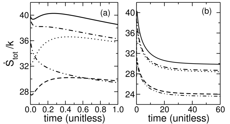Figure 3. Statistical and thermodynamic total entropy production rates on a 6×4 square lattice at kT/J=0.75, during relaxation from the F=0 steady state under field F=4J, for three values of the energy-work coupling constant γ. Graph (a) is an expanded view of the (0,1) time interval of (b)

A non-local-detailed-balance function breaks equality of the thermodynamic and statistical entropy production, causing . Figure 3 shows the difference for the coupling function in(14) with γ=1/2 and γ=1. At γ=0 the statistical and thermodynamic entropy production rates are the same. When local detailed balance is violated, γ>0, the two dissipation rates differ greatly at short time. Subject to an additional assumption, Brey and Prados[40] showed . As Figure 3 shows, the present system satisfies that inequality at short times (Figure 3a) but not at longer times(Figure 3b). The additional condition required by Brey and Prados for the inequality is that the steady state probability distribution be canonical, a condition that does not apply to the DLG.

Solid line: γ=0, so . Dash-dot line: for γ=1/2. Dotted line: for γ=1/2. Dash-dot-dot line: for γ=1. Dashed line: for γ=1.

4. Entropy Production

4.1. Square Lattice

Figure 4 shows the trajectory in (u/J, S_sys/k) from the equilibrium state to the F=4J steady state (solid line). Throughout the trajectory, the bath temperature was kT/J=0.55. The system was initially at equilibrium. Then an F=4J field was applied(t=0) and the master equation was integrated over time to the F=4J steady state. Along the integration path, energy and internal entropy were calculated. The return path in which the system was initially at the steady state under field F=4J is also shown(dashed line). For the return path, the field was reduced from 4J to zero at the initial time.

Figure 4. 6×4 square lattice at kT/J=0.55. Solid line: integration from the F=0 equilibrium state (•) to the F=4J steady state ♦. Dashed line: integration from the F=4J steady state back to the F=0 equilibrium state

The total entropy production rate along the integration path is shown in Figure 5 for the first unit of time integration. The total entropy production rate is not monotone during relaxation to steady state, both falling and rising. The steady state has a lower entropy production rate than states from which it formed, so the F=4J steady state is not a state of maximum entropy production.

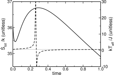Figure 5. The total entropy production rate , solid line, and effective temperature, dashed line, for the initial part of the equilibrium-to-F=4J trajectory shown in Figure 4. The dotted line is the bath temperature, kT/J=0.55

The slope of the trajectory in Figure 4 is an effective temperature, kT_eff/J, because du/dS_sys=T at equilibrium. The slope begins at kT_eff/J=0.55, the bath temperature, at the equilibrium point. As the trajectory approaches the F=4J steady state kT_eff/J reaches 0.50, which is consistent with the interpretation that the field cools the square-lattice driven gas.

4.2. Hexagonal and Triangular Lattices

Trajectories between steady states on a hexagonal lattice are shown in Figure 6, for which the bath temperature kT/J=0.33. Each trajectory has two points where the path turns. At those points the effective temperature T_eff diverges. Approaching the F=0 steady state, kT_eff/J≈kT/J=0.33, as expected. Approaching the F=4J steady state, kT_eff/J≈2.4, which is consistent with the field heating the lattice gas.

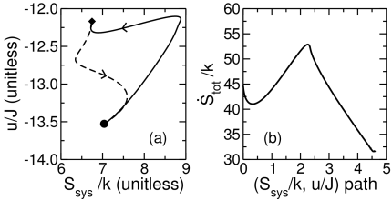Figure 6. Relaxation on a 2×3 hexagonal lattice at kT/J=0.33. Solid line (a and b): integration from the F=0 equilibrium state (•) to the F=4J steady state ♦. Dashed line: integration from the F=4J steady state back to the F=0 equilibrium state. Graph b shows the total entropy production rate versus distance along the path from F=0 to F=4J

However, the overall effect of increasing the field is to lower the steady-state entropy and raise the steady-state energy, so that the overall change cannot be interpreted as effective heating, as can be seen in Figure 6a.

Figure 6b shows that entropy production is not monotone along the trajectory. There is a local maximum and there are two local minima along the path to the F=4J steady state. (The second minimum is not readily apparent in the figure because it is shallow and occurs near the end of the path.) The rate of entropy production at steady state is greater than at the minimum immediately preceding it, and smaller than along much of the path preceding it. Entropy production is neither maximized nor minimized at steady state.

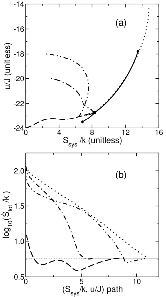Figure 7. 4×3 triangular lattice at kT/J=0.35. Steady states (a): ■ F=J, • F=0 equilibrium, ♦ F=4J. All trajectories in (a) end at the F=J steady state (■). Solid lines: integration from the F=0 equilibrium (•) or the F=4J steady state (♦) to the F=J steady state (■). Dashed line: integration from one configuration having all particles in two columns, Dotted line: integration from the uniform distribution, Dash-dot line: from a 20-bond state, Dash-dot-dot line: from an 18-bond state

Several energy-entropy trajectories on a triangular lattice appear in Figure 7, integrated with a field strength F=J and a bath temperature kT/J=0.35. Figure 7a shows transitions from various states to the F=J steady state. The dotted line is the path from the uniform distribution, in which all configurations have equal probability, to the F=J steady state. The path from F=4J to F=J lies almost along the trajectory from the uniform distribution. Driven steady states on the triangular lattice, at least at this temperature, are along the path to total disorder. The dashed line is the path from a single configuration in which all the particles are in the left two of the four columns of cells.(That initial state was chosen to resemble the broken-symmetry strip that is observed by Monte Carlo simulation on large square lattices.) The remaining two paths originate in states in which all configurations have the same energy, or number of bonds. The dash-dot-dot line begins from a random selection of configurations in which there are eighteen nearest-neighbors (bonds). Its trajectory joins that coming from the zero-entropy single-strip initial state, represented by the dashed line. The dash-dot line originates in a lower-energy twenty-bond group of configurations and follows a distinct route to the steady state.

The rate of total entropy production is in Figure 7b, where the abscissa is the distance along the corresponding trajectory in Figure 7a. The horizontal line shows that the steady-state entropy production is approached on all trajectories. Some paths show non-monotone variation of entropy production, so that the rate of entropy production is neither minimized nor maximized at steady states on the triangular lattice.

The driving field tends to break bonds and increase entropy on the triangular lattice, but it forms bonds and decreases entropy on the square lattice, as is apparent in Figures 4 and 7. These results are consistent with Monte Carlo calculations for large lattices, where single strips are observed on square lattices but only weak ordering is observed on triangular lattices.

5. Kovacs Effect

Prados and Brey[16] describe the Kovacs effect as non-monotonic change of a system property during relaxation of the system from a non-equilibrium state to equilibrium. Commonly, temperature has been the control variable, with relaxation following an abrupt change in temperature. [16,43] The effect is observed as the system relaxes from one steady state to another. A property of the system(e.g., energy, internal entropy) is followed during relaxation. When the property reaches the value it would have been in an intermediate steady state, the control variable(e.g., temperature) is changed to that intermediate value. If the system were internally equilibrated to the intermediate steady state, its property would remain at the intermediate steady-state value and relaxation would be complete. The Kovacs effect is observed when the property continues changing before finally relaxing back to its intermediate steady-state value.

Figure 8 shows typical Kovacs humps in S_sys/k during relaxation to driven steady states. The control variable is field strength rather than temperature. There is also a Kovacs effect when temperature is changed abruptly at fixed field strength, but because the effects found were small no figure showing temperature-induced Kovacs effects is included.

The entropy-time paths of Figure 8 were prepared as follows. The steady state probabilities were calculated at kT/J=0.6 and F=4J. That was the initial state for all five lines. Under zero field, the state relaxed to the equilibrium state. Relaxation in the energy-entropy plane (not shown) followed a path similar to that shown as a dashed line in Figure 4, which is for a slightly lower temperature. Likewise, integration under fields of F=J and F=2J produced the entropy arcs rising toward steady states in Figure 8. To observe the Kovacs effect under F=2J, the F=4J-to-0 trajectory was followed toward equilibrium until S_sys/k=2.70, its F=2J steady-state value. At that time, t=2.42, the field strength was raised from zero to 2J, causing the system to begin relaxing to the F=2J steady state. Figure 8 shows that S_sys/k initially rose, producing the Kovacs hump, before falling back to its steady-state value. To observe the Kovacs effect at F=J, an analogous procedure was followed. The field was raised from zero to F=J at t=10.89 when S_sys/k=7.81, its F=J steady-state value.

Figure 8. Kovacs-like effect on the 6×4 square lattice at kT/J=0.6 beginning from the F=4J steady state at zero time. Solid line, relaxation to the F=0 equilibrium state. Dashed line, relaxation to the F=J steady state. Dash-dot line, relaxation from the F=4-to-0 trajectory to the F=J steady state. Dotted line, relaxation to the F=2J steady state. Dash-dot-dot line, relaxation from the F=4-to-0 trajectory to the F=2J steady state

Considered from the microscopic perspective of trajectories through configuration space, the Kovacs effect is not surprising. The time dependence of probability in configuration space is described by(7). While the control parameters of temperature and field strength are constant, probability evolves smoothly over configuration space. An abrupt change in the field strength(or the temperature) changes the eigenvalues and eigenvectors, which in turn causes a sudden change in the direction of evolution. In a two-dimension energy-entropy projection of the trajectory, as in Figure 4, the direction and speed of the trajectory also change. As the system relaxes into the new steady-state target, a continued change in the macroscopic property(S_sys/k in Figure 8) produces a "Kovacs hump."

6. Summary and Discussion

The rate of entropy production in the surroundings of the lattice gas, , was shown to be the same, whether calculated from probability current in the system or from heat transferred to the bath, as long as there was local detailed balance. In the absence of local detailed balance, the two measures of were unequal. The difference between statistical and thermodynamic was illustrated in Figure 3 by calculations done with a non-local-detailed-balance rate function.

Energy-entropy relaxation paths between steady states on square lattices indicated effective cooling by the external field. That cooling may be interpreted as causing the rise of critical temperature with increasing field strength. Entropy-energy paths for triangular lattices showed a smaller cooling effect. On the triangular lattice, the field increased both S_sys/k and u/J of steady states(Figure 7a), disordering the triangular-lattice gas. Energy-entropy paths on a hexagonal lattice were not simply explained. Hexagonal-lattice relaxation remains a subject for future research.

The results showed that entropy production rate does not vary monotonically during relaxation of gases on the small square, hexagonal and triangular lattices. Maxima and minima of entropy production were observed along relaxation trajectories, so the steady state is not, generally, a state of either maximum or minimum entropy production. According to our observations, the principles of maximum or minimum entropy production at steady state do not apply to the lattice gas when driven upon the small lattices of this work.

An alternative principle for selecting transitions, the principle of maximum second entropy,[13] will be explored in future work. The second or dynamical entropy is the number of configurations connected by a transition between macrostates in a specified time[44] For the driven lattice gas, a macrostate is a set of configurations that share a macroscopic property such as internal entropy. The subject for future study is to explore whether second entropy is maximized along relaxation paths to steady states of the driven lattice gas.

ACKNOWLEDGEMENTS

This research was supported in part by the National Science Foundation through TeraGrid resources provided by the National Center for Supercomputing Applications(cobalt). This work also relied upon computer access granted by the Minnesota Supercomputing Institute of the University of Minnesota. Additional computing resources were provided by the Department of Chemistry and Biochemistry and the Visualization And Digital Imaging Laboratory of the University of Minnesota Duluth. Authors Ford and Zielke gratefully acknowledge support from the University of Minnesota’s Undergraduate Research Opportunities Program and the Department’s Summer Undergraduate Research Program.