-
Paper Information
- Next Paper
- Paper Submission
-
Journal Information
- About This Journal
- Editorial Board
- Current Issue
- Archive
- Author Guidelines
- Contact Us
Research in Otolaryngology
p-ISSN: 2326-1307 e-ISSN: 2326-1323
2017; 6(4): 47-54
doi:10.5923/j.otolaryn.20170604.01

Study the Effect of the Quality Factor of the Transient Evoked Oto-acoustic Emissions (TEOAE)
 Abstract
 Reference
 Full-Text PDF
 Full-text HTML
Adnan AL-Maamury, Dhifaf Ahmed
Al-Mustansiriyah University, College of Science, Department of Physics, Baghdad, Iraq
Correspondence to: Adnan AL-Maamury, Al-Mustansiriyah University, College of Science, Department of Physics, Baghdad, Iraq.
| Email: |  |
Copyright © 2017 Scientific & Academic Publishing. All Rights Reserved.
This work is licensed under the Creative Commons Attribution International License (CC BY).
http://creativecommons.org/licenses/by/4.0/

The effect and role of the quality factor in the nonlinear model was studied in this research. The nonlinear model is one of a set of models that deals with the relationship between frequency and latency of transient evoked otoacoustic emission (TEOAE). Different values of the quality factor were used in non-linear model calculations to determine values which give the best results. For more accurate results, a range of stimulus levels were used. After performing calculations for different quality factor values and stimulus levels, small quality factor values less than 10 show good results for most of stimulus levels, while large values greater than 10 give less accurate results. With regard to stimulus levels, the results were different, with stimulus levels 50, 60 and 70 results are good and accurate. As for the rest of the levels, the results were less accurate, results of stimulus levels 50 dB and 60 dB are better compared to other levels.
Keywords: Quality Factor, Stimulation Levels, Nonlinear Model, TEOAEs, Latency, Frequency
Cite this paper: Adnan AL-Maamury, Dhifaf Ahmed, Study the Effect of the Quality Factor of the Transient Evoked Oto-acoustic Emissions (TEOAE), Research in Otolaryngology, Vol. 6 No. 4, 2017, pp. 47-54. doi: 10.5923/j.otolaryn.20170604.01.
1. Introduction
- Presence of the otoacoustic emissions on the basis of mathematical models of cochlear nonlinearity predefined by Thomas Gold in 1940s. However, one was not able to measure OAEs up to the year 1970s, when technology researchers allow recording these responses by microphones very sensitive placed in the external hearing channel [1]. OAE is the first to experimentally interpreted in 1978 by David Kemp [2], which was discovered the OAEs measurement in the ear canal arises from the nature of the secondary process active in hearing [3], And showed that otoacoustic emissions are generated inside the ear in human cochlea by having a different number of mechanical and cellular reasons [4, 5]. Narrow band otoacoustic emissions will respond to acoustic stimulation when there is evoked emissions or non-respond to acoustic stimulation in the absence of spontaneous emissions [6].In recent years, the discovery of acoustic emission has led to expand our understanding of the process of hearing. Knowledge of OAEs resulted in explanation of certain physiological and anatomical findings that were either newly discovered or did not explain for several years. So, the discovery has led to a good understanding of the work of cochlear system of the IHCs [7]. Otoacoustic emissions that are produced by the low-level cochlea are measured by sending the sounds to the middle ear through a probe that contains a small microphone and a loudspeaker that converts the resulting sound into digital and is processed by an electronic device placed in the ear canal. The sounds are transferred to the external ear [8]. As it's known that OAEs are generated from two distinct mechanisms: an active non-linear element included the OHCs, and passive linear reflection of the travelling wave along the basilar membrane. Talmadge succeeded in applying a model of the cochlear several years after the discovery of otoacoustic emissions, which is a physiological process produced in the active mammalian cochlea. According to this model, sound waves located along the basilar membrane play an important role in generating spontaneous otoacoustic emissions that transmit the acoustic signal to the channel External ear through middle ear [10]. Through cochlea models, acoustic emissions are generated and sent back with conditions the resistance transverse of the resonant ton topically [11]. Based on the knowledge of the mechanism and behavior of the outer hair cells in the cochlea, several models of the feedback mechanism have been developed. These models, whether non-local and non-linear, should be comprehensive in the cochlea [13]. In the past decades, the external hair cells that are associated with the basilar membrane and tectorial membrane have been tested and comparing this pairing with experimental data which resulted in a high number of free parameters that reached a high degree of complexity [14]. Theoretical interpretation of experimental data helps the researcher to provide new diagnostic techniques for the design and improvement of cochlear function. Cochlear models are a useful tool for understanding the basic cochlear physiology and their use in running numerical experiments as an input to the model from feeding a particular type of stimulus. These experiments were compared with the real analog experiments and the results were compared in two stage: stage I, refining and validating the model; stage II, using the model to predict cochlear behavior and access to experimental techniques beyond their range [15, 16]. Using a limited number of free parameters, many cochlear models, including active, linear and nonlinear terms, have been discussed to plan the active feedback mechanism of the cochlear function. Linear models in the frequency domain can be effectively solved using numerical and analytical approximations at low computational costs. The same feature applies to nonlinear models which are a major feature of the physiology of cochlear and can be solved using the disorder system [17]. Finally, the discovery of OAEs Allows hypotheses are introduced to account for many of the psychoacoustical phenomena including the microstructures of behavioral sensitivity and loudness improve which were vague in terms of traditional models of the auditory system [9].
2. Methods
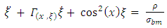
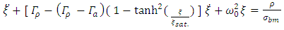
- The description of a first approximation for eq.(1) and eq.(2), the simple passive cochlea model is used with one dimension [14]. Model used in this work is the nonlinear and the nonlocal. As in Adnan (2015) [18], Moleti (2009) [14] and Elliott (2007) [19], the main equations are described as follows:
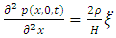 | (1) |
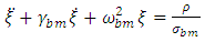 | (2) |
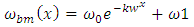 | (3) |
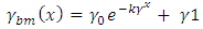 | (4) |
 | (5) |
 | (6) |
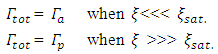
 ) as following:(1) When
  This means
  So
So 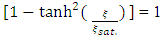 Equation (6) becomes
 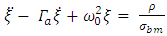 | (7) |
 (2) When
  So the value of
 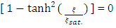 Equation (6) becomes:
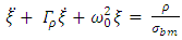 | (8) |

 | (9) |
 The local passive quality factor
 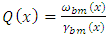 | (10) |
 and
and  ,
,  | (11) |
 , so that the maps of equations (3, 4 and 10) do not clearly break the scale fixed symmetry, where
  is a constant [20].
3. Results and Discussion
- One of models that studies the relationship between frequency and latency of otoacoustic emission is nonlinear model. The purpose of this research is to improve the results of the calculations of the nonlinear model and to obtain more accurate results. The quality factor is one of the most important factors in the nonlinear model. In order to obtain the best results, a series of calculations were performed using the nonlinear model using different stimulus levels (30, 40, 50, 60, 70, 80 and 90) dB.For each stimulus level of this group, the calculations were performed for a set of quality factor (2, 4, 6, 8, 10, 12, 14, 16, 18 and 20).The purpose of this series of calculations is to conduct a comprehensive survey of the values of the quality factor in order to determine the most accurate results of the otoacoustic emission, especially the relationship between frequency and latency.The results were obtained in this work are classified as follows:1 – Stimulus level 30 dBThe results were obtained in this part of the calculations by using the stimulus level 30 dB with all the values of the quality factor, which are 10 cases.Results are different, including fine results and less accurate results.The results obtained using the quality factor values (2, 4, 6 and 8) are good and accurate, while other results are less accurate.Figure 1 shows the relationship between the frequency and latency of the otoacoustic emissions of the stimulus level 30 dB, which includes four different cases.The four cases represent four curves which are as follows:1- The first curve represents the relationship between frequency and latency of stimulus level 30 dB using quality factor value is 2.2- The second curve represents the relationship between frequency and latency of stimulus level 30 dB using quality factor value is 4.3- The third curve represents the relationship between frequency and latency of stimulus level 30 dB using quality factor value is 6.4- The fourth curve represents the relationship between frequency and latency of stimulus level 30 dB using quality factor value is 8.
 | Figure 1. Shows the relationship between the frequency and latency of the transient evoked otoacoustic emission (TEOAE), for the stimulus level 30 dB and quality factor (Q= 2, 4, 6, 8) |
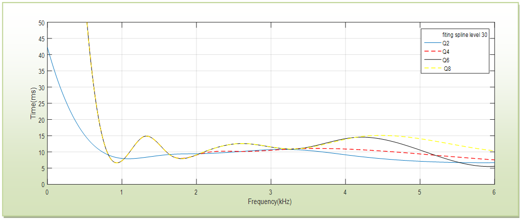
 | Figure 2. Shows the relationship between the frequency and latency of the transient evoked otoacoustic emission (TEOAE), for the stimulus level 40 dB and quality factor (Q= 2, 4, 6, 8) |
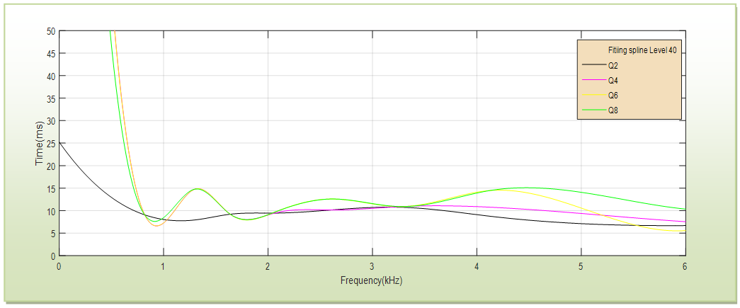
 | Figure 3. Shows the relationship between the frequency and latency of the transient evoked otoacoustic emission (TEOAE), for the stimulus level 50 dB and quality factor (Q= 2, 4, 6, 8, 10, 12, 14, 16, 18, 20) |
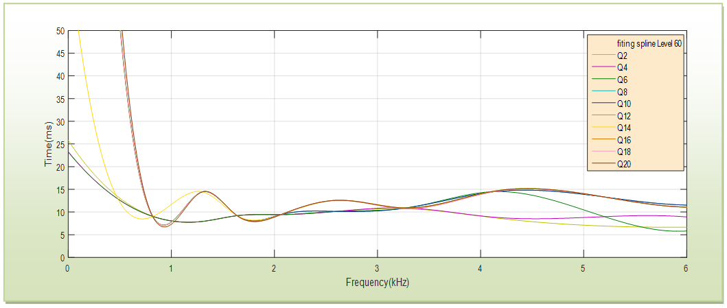 | Figure 4. Shows the relationship between the frequency and latency of the transient evoked otoacoustic emission (TEOAE), for the stimulus level 60 dB and quality factor (Q= 2, 4, 6, 8, 10, 12, 14, 16, 18, 20) |
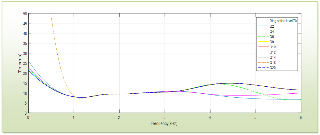 | Figure 5. Shows the relationship between the frequency and latency of the transient evoked otoacoustic emission (TEOAE), for the stimulus level 70 dB and quality factor (Q= 2, 4, 6, 8, 10, 12, 14, 18, 20) |
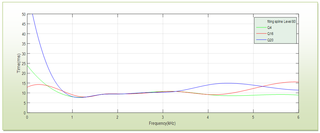 | Figure 6. Shows the relationship between the frequency and latency of the transient evoked otoacoustic emission (TEOAE), for the stimulus level 80 dB and quality factor (Q= 4, 16, 20) |
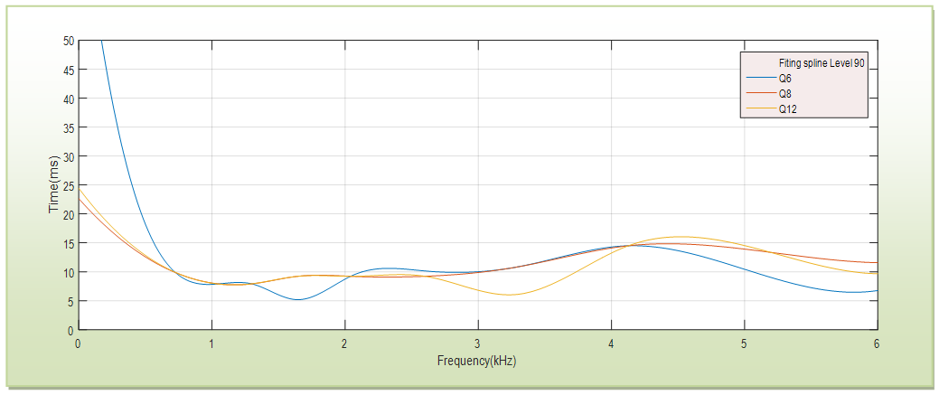 | Figure 7. Shows the relationship between the frequency and latency of the transient evoked otoacoustic emission (TEOAE), for the stimulus level 90 dB and quality factor (Q= 6, 8, 12) |
4. Conclusions
- Based on the results obtained in this work with respect to the effect of the quality factor and stimulus level on the accuracy of the results of the otoacoustic emission, we conclude that the use of the low values of the quality factor in the non-linear model produces better results and more accurate than the high values. These results are compatible with most stimulus levels, while with high values give different results and less accuracy.As for the stimulus levels, the results given were mixed, where the results are good with low quality factor and vary with high values and the best and accurate results were stimulus levels 50, 60 and 70 dB. The results obtained in this work are consistent with previous studies [22-25].
Symbols
- BM is the basilar membrane x is the longitudinal coordinate along the BMt is the time.p is the differential fluid pressure on the BM
 is the fluid density
  is the (BM) transverse displacement at the longitudinal position (x) and time (t)
 dissipation constant of the local BM
 is the BM of the surface density
 the resonance frequency of the local BM.