1. Introduction

A review of the theoretical models of light irradiation and collection in solar concentrators (SC) was presented in the first part of this work [1]. In the second part [2], we presented the application of these models to nonimaging SC of the type 3D-CPC (Three-Dimensional Compound Parabolic Concentrator) irradiated by direct and collimated beams, whereas in the third part [3] the same models were applied to SC irradiated by direct and lambertian beams. In this paper, we continue the analysis of the optical properties of 3D-CPC irradiated by the direct method with collimated beams. The purpose of this work is to obtain maps of the entrance opening carrying the information of the number of reflections made by transmitted and reflected rays. These maps are useful, as they give local information on the transmitted and reflected rays and in the present work said maps will be elaborated at different incidence angles of the parallel beam at the input of the SC.

In the paper by Hinterberger and Winston [4] we have the first appearance of a nonimaging concentrator, at the time called “light funnel”, precursor of the modern CPC. In that work, Hinterberger and Winston were trying to collect the most efficient Čerenkov light to convey it to a photomultiplier. Later, Winston, with other authors, developed a complete and comprehensive theory of nonimaging concentrators, which has found a large spread in the field of concentrating solar power, both for thermodynamic and photovoltaic applications [5-8]. The paper by Hinterberger and Winston simultaneously shows maps of the entrance opening of the funnel, detailing the regions corresponding to certain numbers of reflections made by the transmitted rays. The maps were obtained at different incidence angles of the parallel beam, all the angles being smaller than the acceptance angle of the funnel, . We know that a light funnel like that one collects light with a unitary efficiency up to the acceptance angle, apart from some losses due to absorption on the internal walls. Then the maps shown by Hinterberger and Winston are essentially maps of number of reflections made by transmitted rays, as only few reflected rays are involved. The light funnel of Hinterberger and Winston behaves like a modern 3D-CPC irradiated at , where is the symbol hereafter used to indicate the acceptance angle of the concentrator under direct and collimated irradiation. The incidence angles used by Hinterberger and Winston in [4] were precisely: = 0.0°; 5.0°; 7.5°; 10.0°; 12.5° and 15.0°. The maps show regions with number of reflections of 0, 1, 2, 3, 4, 5, etc., and this number increases moving towards the edge of the funnel opening. The region with zero number corresponds to rays transmitted directly to the output, where the photomultiplier is located. When they observed some thin “failure zones” corresponding to the few detected back-reflected rays. The maps by Hinterberger and Winston are of considerable theoretical interest because they help to understand what happens to the rays entering each point of the entry aperture of the funnel.

The simulations made by Hinterberger and Winston in [4] were carried out by using Monte Carlo techniques. They were featured later in more elaborated form in the works [6-8] where they have been applied to a CPC with .

The aim of the present study is to develop maps of transmittance/reflectance of the kind displayed by Winston in publications [6-8], but made by following different methods of simulation. In the previous works [2, 3] we analyzed a 3D-CPC with ; in this work, we will continue to report results obtained on this CPC. With our method, maps relating to transmitted rays are obtained by irradiating inversely the CPC with Lambertian beams applied to the output opening, whereas the maps relating to the reflected rays are obtained by irradiating directly the CPC with Lambertian beams applied to the input opening.

2. The Compound Parabolic Concentrator (CPC)

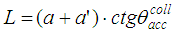
The CPC is a reflective concentrator with a profile obtained by the combination of two parabolas and is characterized by a step-like transmission efficiency allowing the efficient collection of light from 0° to a maximum angle of incidence, the acceptance angle , where the suffix “coll” means collimated beam irradiation. Fig. 1 shows the 3D-CPC used in our simulations. The 3D-CPC, with , is the same used in the previous papers of this series [2, 3] and is shown in Fig. 1.

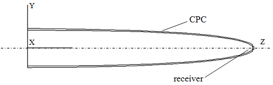Figure 1. Longitudinal cross sections of the “Three-Dimensional Compound Parabolic Concentrator” (3D-CPC) simulated in this work. The angle of acceptance at a parallel beam is

The CPC is characterized by a maximum angular divergence of rays at exit aperture equal to 90° when the incidence angle is equal to the acceptance angle. Only two independent parameters are required to define its shape, among the five appearing in the following equations [2-8]:

(1)

(2)

(3)

where L is the length of the CPC, f is the focal length of the parabolic profile, a is the radius of input aperture and a’ is the radius of output aperture. Therefore, we have for the CPC with = 5°: L = 150 mm, f = 1.14 mm, a = 12.035 mm, a’ = 1.052 mm.

In the previous works [2, 3], the CPC was modified only in the reflectivity parameter of the internal wall, which was varied between 1 (ideal behavior) and 0.8, to simulate the effective reflectivity of real metal surfaces, such as, for example, silver or aluminum. The same thing has been done here.

3. The Simulation Methods

3.1. Maps of Number of Internal Reflections

When an ideal CPC is irradiated directly with a parallel beam inclined by an angle of with respect to the optical axis of the CPC, the input flux is distributed between a transmitted flux and a back-reflected flux , in such a way that:

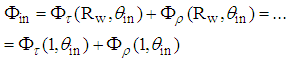(4)

If the CPC is real , the internal wall will absorb a portion of the input flux, which will be now distributed among three components ( is kept constant):

(5)

When we move from the ideal to the real situation, both the transmitted and the reflected beams will suffer attenuation that will be stronger the higher the number of reflections made by the rays on the inner wall of the CPC. Then, the single-beam at input, of power , for example one of the transmitted ones, will be attenuated, after reflections, and its output flux will be:

(6)

But the attenuation experienced by a ray, whether it is intended to be transmitted or reflected, will also depend on the impact point P on the entrance opening, so not every ray transmitted or reflected will experience the same attenuation. Hence the need to distinguish, on the plane containing the entrance opening, regions crossed by rays that are transmitted or reflected after a fixed number of internal reflections. For reasons of continuity, is clear that, if a beam entering at a point P of the CPC entrance opening is transmitted after reflections, there will exist a surrounding of this point through which rays having the same number of reflections will pass. The borders of this region will be determined by those rays striking the rim of the CPC exit opening.

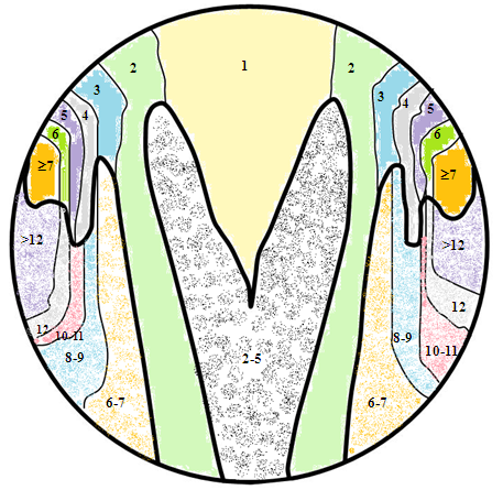
Therefore, fixed a value of , the planar surface overlapping the input opening of the CPC can be divided into different regions, each one characterized by a defined number of internal reflections made by transmitted or reflected rays. But, considering that the path of a transmitted beam will never be superimposed on that of a reflected one, the entrance opening area will be divided into regions crossed only by rays to be transmitted and regions, distinct and adjacent to the first ones, crossed only by beams to be reflected. There will be no regions crossed by simply absorbed beams, as the absorption involves only the subtraction of a part of the transmitted or reflected flux. Only in the case of very low wall reflectivity, or very large number of reflections of the beam, we could consider regions of absorbed rays, but this is not generally the case in practice. It is also evident, from what we have learned about the behavior of a CPC [2-8], that only the rays that enter the CPC near the edges are more likely undergoing a higher number of reflections. Given these considerations, we illustrate now a typical map of entrance opening of a 3D-CPC with distinct regions crossed by the rays that undergo a defined number of internal reflections before being transmitted or reflected. An example of this type of map is shown in Fig. 2: a 3D-CPC with = 10° is irradiated with a parallel beam inclined by from top to bottom [6-8].

The regions of transmitted rays are labeled by n = 0, 1, 2, 3, … and the ones of reflected rays by m = 2, 3, … where n and m are the number of reflections made by transmitted and reflected rays, respectively. In Fig. 2, m is preceded by the letter F, which stands for “Failure”, meaning “failure to being transmitted”. Being , we are in a situation with and so half of rays are transmitted, half are reflected, as it can be seen from the fact that in the map the white regions and the gray-colored ones have the same extension. We are near , then some rays are back reflected after two or three reflections (there are no rays rejected after just one reflection, because of the geometry of the 3D-CPC [2]). 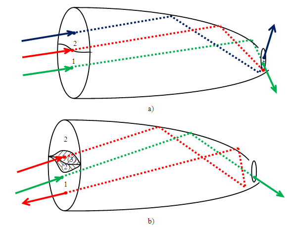To find the local value of , with P as entry opening point, it is necessary to produce in any way the image of the CPC exit opening, as the boundaries of the regions of transmitted rays are nothing more than distorted images of the exit aperture seen after various number of internal reflections [6-8]. Moreover, the failure regions, that is the regions of back-reflected rays, appear as a splitting between these boundary regions. For example, the regions of failure after two and three reflections appear in the diagram of Fig. 2 as a split between the regions of transmission after one and two reflections. This confirms the principle that rays meeting the rim of the exit aperture are at the boundaries of failure regions [6-8]. Each split between regions of transmission after n and n + 1 reflections produces two failure regions, characterized by m = n + 1 and m = n + 2 reflections. An example of raytracing applied to a map of number of reflections is shown in Fig. 3. Figure 3a shows the transition from a region n = 1 to a region n = 2, with two transmitted rays and one ray, that one crossing the border between the two regions, that hits the rim of the exit opening. In Fig. 3b the input rays are more inclined and this determines the splitting of the border between n = 1 and n = 2 regions and the appearance of new failure regions (hatched in the figure) with m = 2 and m = 3. The rays crossing these regions are back-reflected.

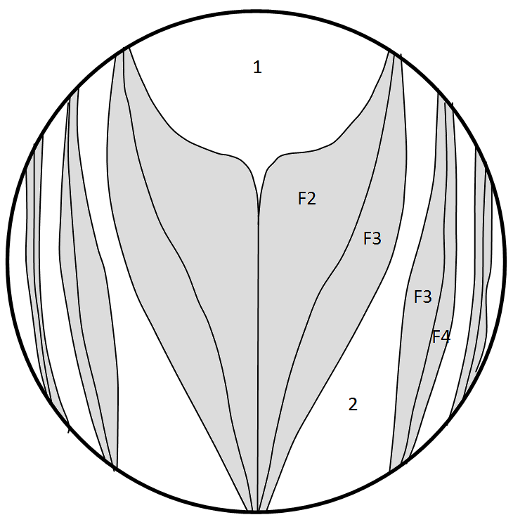Figure 2. Draft of a map reporting the patterns of accepted and rejected rays at the entrance opening of a CPC with 10° acceptance angle [6-8]. The entrance opening is seen from above with incident rays sloping downward at 10° incidence. Rays entering areas labeled n are transmitted after n reflections; those entering the gray-colored areas labeled Fm are turned back after m reflections. The map shows, as an example, only few regions with low n and m values

Figure 3. Simulations of some rays crossing different regions of the entrance opening of the CPC. a) Here we have two adjacent regions with n = 1 and n = 2. The green ray, crossing the white region n = 1, is transmitted after 1 internal reflection, whereas the blue ray, crossing the white region n = 2, is transmitted after 2 internal reflections. The red ray, incident on the border between the two white regions, impacts on the rim of the exit aperture and is scattered towards an undefined direction. b) Here the rays are incident at a greater angle on the entrance opening. This determines the splitting of the border line between n = 1 and n = 2 regions in two hatched regions with m = 2 and m = 3. The green ray, crossing the white region n = 1, continues to be transmitted after 1 internal reflection, whereas the red ray, crossing the hatched region m = 3, is back reflected after 3 internal reflections

3.2. Simulation Schemes

For simplicity, we start reviewing the case of an ideal concentrator . The map of this concentrator is divided into two types of regions: white regions crossed by transmitted rays and hatched regions crossed by reflected rays. Each region is characterized by a number (put in parentheses for regions of reflected rays) indicating the number of reflections made by a beam transmitted or reflected before exiting the concentrator. As suggested by Winston et al. [6-8], we can delineate these regions by tracing rays in a reverse way from the exit aperture. To obtain maps of as distorted images of the CPC exit opening viewed from the entrance opening, it is necessary to irradiate the exit opening in the inverse mode by a Lambertian source of 90° divergence and to collect the rays inversely transmitted at a fixed angle , the same angle of the incident rays. This is possible thanks to the principle of reversibility, establishing, for a non-polarized light beam subjected to reflections and/or refractions on surfaces and/or interfaces in which diffusive or diffractive phenomena are absent, the same attenuation in both directions of the optical path [1, 9].

Therefore, the map of the exit opening can be obtained irradiating it with a Lambertian source (constant radiance in all directions) in such a way as to provide all possible rays in the reverse direction, including those which in direct mode would cross the input opening at angle , and collecting on a far screen the rays exiting from the input opening at angle.

Fig. 4 shows the scheme for measurement of the inverse image of the CPC. If we want to obtain the image of the CPC at angle , the CPC is tilted by an angle with respect to the optical axis (counterclockwise, CCW, rotation of angle around the x axis); at distance x₁ there is the diaphragm+lens system and at distance x₂ from the lens there is the screen (a perfect absorber) on which the image is formed. By changing the tilting of the CPC, we will get the different images of the CPC for the different values of . The simulations made with the scheme of Fig. 4 do not give the number of reflections, but only the map of intensity of the rays inversely transmitted at the angle and crossing the white regions of Fig. 2. If the wall of the CPC is a perfect mirror , for example, the rays undergoing a different number of internal reflections would exit the CPC with the same intensity, due to absence of optical loss and therefore they would not give any detail about the number of reflections made. Therefore, to highlight the number of internal reflections, we need to start from Eq. (6), which tells us that the information on the number of internal reflections is carried out by the intensity of rays at the end of the optical path. If we apply Eq. (6) twice at two different wall reflectivities, it is easy to extract the number of reflections after comparing the two corresponding intensities. This was, in effect, the method largely used by us in previous works to calculate the average number of reflections inside the CPC at different operating conditions [2, 3]. In the present case, to draw a map of and , we need to discriminate between the different points of the CPC entrance aperture.

The value of at each point of the CPC input aperture is obtained applying Eq. (6) to two close values of , 1.0 and 0.8, and the following equation [2, 3]:

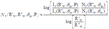(7)

where:

: CCW tilting angle of the CPC around x-axis;

: Intensity of image at the point, on the screen, corresponding to the point P of the input opening of the CPC;

: total number of rays collected on the screen;

: two close values of wall reflectivity.

In Eq. (7), the intensity of the transmitted beam incident on point P at the input opening of the CPC is equivalent, thanks to the principle of reversibility that we discussed above, to the intensity of the beam transmitted backwards along the same optical path when we irradiate in reverse mode the exit aperture; this intensity can be extracted from the image of the CPC formed on the screen far away (see Fig. 4). The inverse irradiation of the CPC is at the base of the “inverse method” of characterization of SC, developed by us since 2007 [1, 9-32], and was introduced as an alternative to the traditional, more complex and slow, “direct method” of characterization [1-3, 11, 14, 15, 17-20, 22, 23, 25, 27, 28, 33-37].

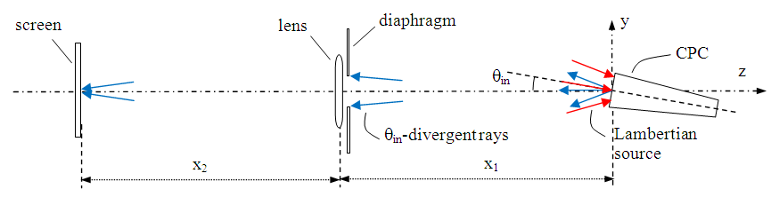
Fig. 4 shows the scheme of the simulation followed to obtain the map of , the number of reflections of local transmitted rays. This map contains, in principle, only information about the white regions of the map (see Fig. 2). In this map, the regions crossed by the back-reflected rays should result empty.

To obtain the map of the gray-colored regions (see Fig. 2), which are those crossed by the input rays back-reflected from the CPC, we need to simulate the reflected rays in the reverse direction, that is impinging on the entrance opening. To do this, we irradiate in a direct way the entrance opening of the CPC with a Lambertian source (which emits rays in all the possible directions with the same radiance) and then we reproduce the image of the CPC on the absorbing screen. Fig. 5 shows the new scheme, where we have moved the Lambertian source from the exit opening to the entrance opening. The simulation scheme represented in Fig. 5 will give us the gray-colored regions of the map.

To obtain the number of reflections to be assigned to the different gray-colored regions, we apply an equation like to the one used to obtain :

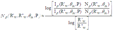(8)

where:

: CCW tilting angle of the CPC around x-axis;

: Intensity of image at the point, on the screen, corresponding to the point P of the input opening of the CPC;

: total number of rays collected on the screen;

: two close values of wall reflectivity.

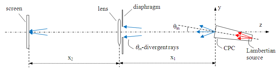Figure 4. Scheme of the simulation method adopted for obtaining, at θin angle, the intensity image map of the CPC carried out from the transmitted rays. The blue color of transmitted rays indicates that the red source rays undergo an attenuation inside the CPC, as an effect of internal reflections, when the wall reflectivity is not unitary

Figure 5. Scheme of the simulation method adopted to obtain, at θin angle, the intensity image of the CPC carried out from the back-reflected rays. The blue color of the back reflected rays indicates that the red source rays undergo an attenuation inside the CPC, as an effect of internal reflections

3.3. Image Formation

The following lens was chosen for the schemes of Figs. 4 and 5: Schott BK7 biconvex lens, of 10 mm thickness and 500/-500 mm radii. To appropriately size the distances in the diagrams of Figs. 4 and 5, that is to obtain a correct image of the entrance opening of the CPC on the screen, we made at first some tests of image formation with a simple prism placed at z = 0, and with dimensions: Δx = 1 mm, Δy = 5 mm, Δz = 1 mm, as shown in Fig. 6a.

To keep low the angular divergence of the rays collected by the lens and focused on the screen, we choose a high value of x₁, 995.5 mm, and a small aperture of the diaphragm, 12 mm of radius (the same of the entrance opening of the CPC), hence an angular resolution of approximately 0.7°. We first measured the focal length of the thin lens by applying a parallel light source on the face of the prism directed along the –z direction (see Fig. 6a), obtaining the value f = 485.24 mm. Applying the thin lens equation: 1/f = 1/x₁ + 1/x₂, we obtained the distance between the lens and the screen, x₂ = 945.7 mm. Then we did a simulation to get the image of the prism using the scheme of Fig. 4 or 5. The image of the prism was obtained by applying to its face, directed towards –z direction, a Lambertian source of light with 0.7° divergence, as it is shown in Fig. 6b and 6c. The image of the prism is a good reproduction of the object, consequently we proceeded to replace the prism with the CPC, placing it as shown in Figs. 4 and 5, that is with its entrance opening centered on the origin of the axes and with its optical axis rotated CCW by an angle of around the x axis.

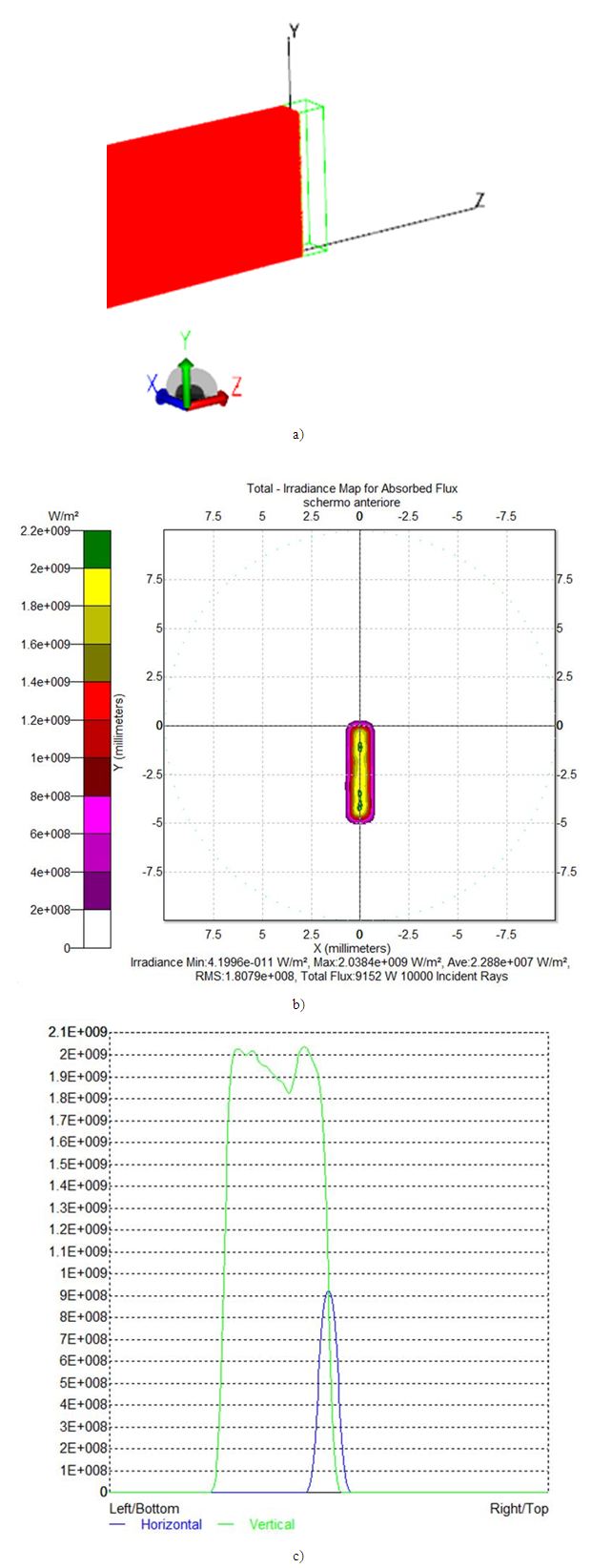Figure 6. (a) Raytracing of a parallel beam from a source prism to find the focal length of the lens. (b) Image of the prism obtained by a source emitting Lambertian light with 0.7° divergence towards the –z direction. (c) x-y profiles of the image

4. Simulation Results

4.1. Maps of Transmitted Rays

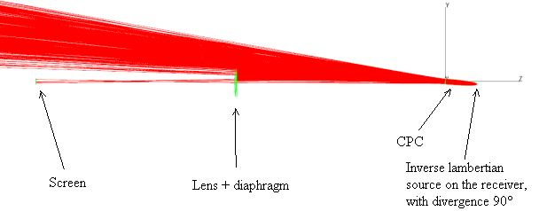
We start applying the simulation method illustrated in Fig. 4 to obtain the map of transmitted rays. Let us consider first the simplest case, the one with = 0°. Fig. 7 shows an example of the raytracing of the inverse lambertian source applied to the exit opening of the CPC. It is possible to note how the inversely projected rays to the left from the entrance opening of the CPC are only slightly divergent, being that the maximum angular divergence matches the angle of acceptance, which is 5° [9-32]. Fig. 8a shows the map of the irradiance obtained on the screen when the wall reflectivity is 1.0, and Fig. 8b shows the corresponding radial profile. This map was obtained by imposing the cylindrical symmetry to improve the signal-to-noise ratio. The simulation was carried out with 500k rays. Apart from the thin central peak, due to the limited number of rays used, the intensity profile is flat, as expected. Fig. 9a shows the map of the irradiance obtained on the screen when the wall reflectivity is reduced to 0.8, and Fig. 9b shows the corresponding radial profile. 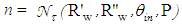To obtain the map of number of reflections , we apply Eq. 7, where is the irradiance map of Fig. 8a and is the irradiance map of Fig. 9a. Fig. 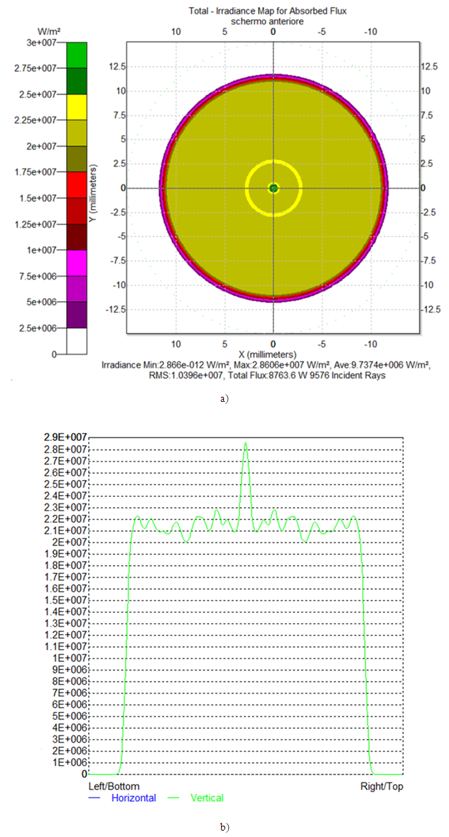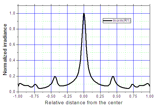10 shows the map of number of reflections n = made by the transmitted rays. The areas with different number of reflections are distinguished by different colors. From Fig. 10 we can see that in most of the central regions of the entrance opening the number of reflections is one and increases going towards the periphery. The small central region with n = 0, referred to the rays that pass through the CPC without reflections, remains unresolved.

This is a consequence of the fact that the inverse rays at the output of the CPC that are collected by the system diaphragm+lens+screen have a slight divergence (≈0.7° instead of 0°). The annular regions with n > 1 shrink as n increases from 2 to 6, while the annular regions between 7 and 25 are grouped in the single green olive region. The radial profile of the map of Fig. 10 is shown in Fig. 11 (black curve).

It is interesting to compare the profile of n relative to the rays incident on the entrance opening of the CPC (black curve in Fig. 11) with that relative to the rays incident on the exit opening of the CPC (red curve in Fig. 11), when the rays belong to the same parallel beam incident at 0° at the input of CPC. The red curve of Fig. 11 is derived from [2] (see red curve in Fig. 11 of this reference).

Although these two profiles belong to different apertures of the CPC, the entrance and the exit ones, they closely resemble. The rays incident at 0° on the entrance opening are uniformly distributed, while those incident on the exit opening are for the most part concentrated in the center (see Fig. 12), nevertheless, the spatial distribution of n, average number of reflections, on the two openings is very similar. Therefore, the distribution of n, not of the flux density, is transferred, almost unchanged, from the entrance to the exit opening. This is really an interesting and unexpected result.

To obtain the map of n at θ_in= 5°, the CPC was rotated by 5° CCW around the x axis, while keeping the center of the entrance opening in the origin of the axes, and two new simulations were made at and , following the scheme of Fig. 4. A rough example of the raytracing diagram of inverse rays, in this case, is shown in Fig. 13. The true simulations were carried out with 4M rays and ≈12h running time.

Figure 14a shows the map of the irradiance obtained on the screen when the wall reflectivity is 1.0. This map cannot be symmetrized to improve the signal-to-noise ratio, as it no longer has a cylindrical symmetry. Then, the radial profile cannot be shown. The white areas in the maps of Fig. 14 correspond to those of the CPC entrance opening whose incident rays are back-reflected and cannot reach the exit opening. As consequence, those rays do not appear among the inverse rays produced by the Lambertian source placed on the exit opening of the CPC. In the map of Fig. 14a, the most intense regions are those where more rays converge, being that the rays do not undergo optical attenuations. This transmission map should show, in principle, a uniform intensity throughout the area affected by the passage of the transmitted rays, because it should reproduce the map of irradiance distribution which could be measured intercepting a direct and uniform, parallel beam, incident on the CPC, by a plane orthogonal to its direction of propagation. The intensity unevenness, in the area affected by the passage of the transmitted rays, is just an effect of the low angular resolution of the simulations.

Differently from the map of Fig. 14a, the intensity of the different zones in the map of Fig. 14b depends on the attenuation that the incident rays undergo as an effect of the optical loss on the CPC internal wall. From the two maps of Fig. 14 we can see that the reduction of the wall reflectivity from 1.0 to 0.8 produces a general reduction of the intensity on the screen, as expected.

From the maps of Fig. 14 we can also see that most of rays join the upper part of the screen. Some of them contribute to form vertical bands of intensity in the lower part of the map. This is a direct consequence of the unevenness of the flux distribution on the exit opening of the CPC (where is placed the receiver), when it is irradiated in direct mode by a collimated beam [11, 17, 19, 23, 29, 34], in contrast to the uniform, inverse, Lambertian irradiation applied here to the exit opening. We also notice that the white area, the one concerning the back-reflected rays, remains well-defined and unaffected by the reduction of .

To obtain the map of number of reflections , we apply Eq. 7, where is the irradiance map of Fig. 14a and 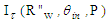is the irradiance map of Fig. 14b. In Fig. 15 it is shown the map of the average number of reflections made by the transmitted rays. The different areas of the map are distinguished by different colors and labeled with the corresponding number of internal reflections.

From Fig. 15 we can see that the 5° rotation of the CPC has the effect of cutting in two the annular regions with n > 2 shown in Fig. 10, separating them, while the region with n = 2 remains connected in the lower part of the map and the central region of the map with n = 1, is stretched and moved upward. As in the case of the map of Fig. 10, also here the annular regions with n ≥ 7 are grouped in the zones of magenta color. The map of Fig. 15 has a topological aspect resembling that of Fig. 2 for the triangular shape of the n = 1 region and for the V shape of the n = 2 region. However, the map of Fig. 15 is not the final map that we look for; this one will be obtained only after the simulations of the map of reflected rays.

Since the maps of irradiance on the screen traced until now should reproduce the distorted images of the CPC exit opening as viewed through the CPC entrance opening, we tried a new simulation carried out by illuminating in reverse mode, instead of the entire exit opening area, only a very narrow annular ring of it containing its edge (with minor radius of 1 mm and major radius of 1,052 mm). The simulation was made always using a Lambertian source with the CPC CCW-rotated by 5° and with a wall reflectivity R_w = 1. In this way, we expect to get a map of intensity in which are highlighted the contours of the regions with different n, as obtained in Fig. 14a.

Figure 16 shows the simulation result obtained after a raytracing with 3M rays. Comparing this map to the one of Fig. 14a, we note that not only the contours are now more defined, but also that areas with greater intensity appear at the edges. These regions are the most distorted images of the exit opening and correspond to a higher number of reflections made by the transmitted rays.

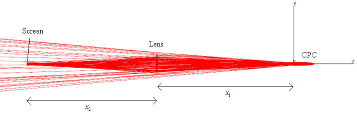Figure 7. Raytracing obtained irradiating in inverse mode the exit opening of the CPC by a Lambertian source. The CPC is oriented along the z direction, corresponding to θin= 0°

Figure 8. Symmetrized map (a) and corresponding radial profile (b) of the irradiance measured on the screen of Fig. 4 when the CPC is oriented at θin= 0° respect to the z axis. Wall reflectivity R’w = 1.0

Figure 9. Symmetrized map (a) and corresponding radial profile (b) of the irradiance measured on the screen of Fig. 4 when the CPC is oriented at θin= 0° respect to the z axis. Wall reflectivity R’’w = 0.8

Figure 10. Symmetrized 2D map of the local distribution, on the entrance opening of the CPC, of the number of reflections the rays incident at 0° make on the internal wall of the CPC before being transmitted to the exit opening

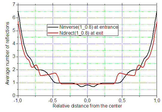Figure 11. Radial profile of the average number of reflections of a parallel beam at 0° incidence. The black curve represents the average number of reflections made by the transmitted rays incident on the entrance opening of the CPC. The red curve represents the average number of reflections made by the transmitted rays incident on the exit opening of the CPC (the receiver). The relative distance r is calculated with respect to a = 12.035 mm, the radius of entrance opening, for the black curve and with respect to a’ = 1.052 mm, the radius of exit opening, for the red curve

Figure 12. Irradiance profile of the flux at the exit opening (receiver) of the 3D-CPC, irradiated by a collimated beam parallel to the optical axis

Figure 13. Raytracing obtained irradiating in inverse mode the exit opening of the CPC by a Lambertian source. The CPC is oriented at θin= 5° off the z direction, counterclockwise around the x axis

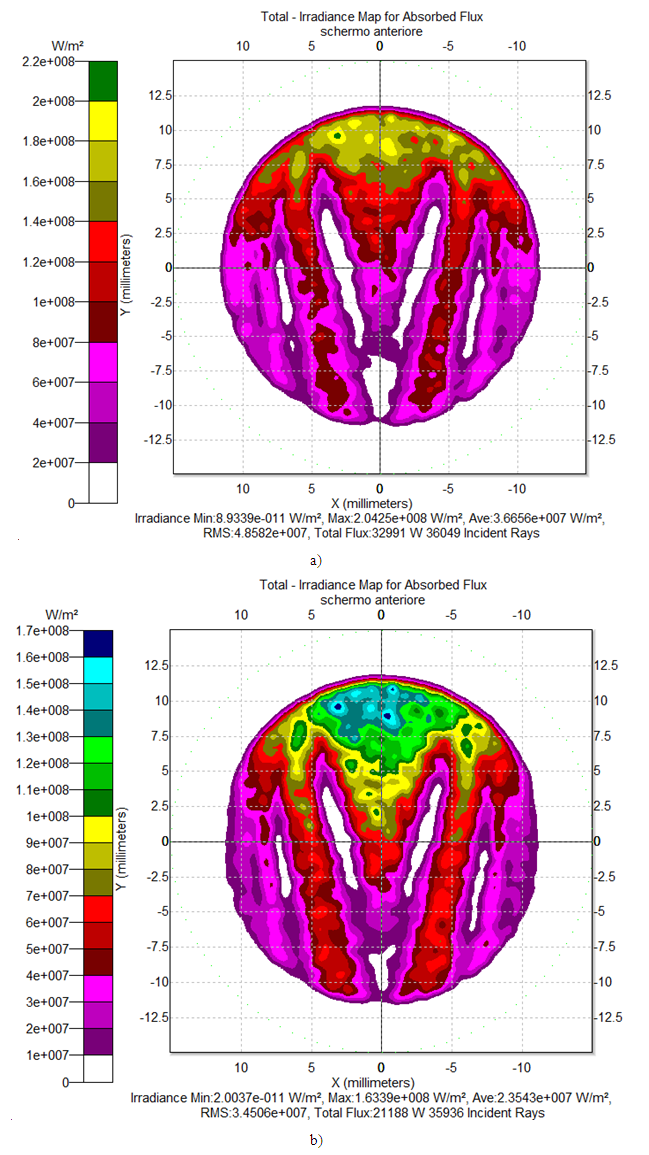Figure 14. Maps of the irradiance measured on the screen of Fig. 4 when the CPC is oriented at θin= 5° respect to the z axis. a) Wall reflectivity R’w = 1.0; b) wall reflectivity R’’w = 0.8

Figure 15. Map of the CPC entrance opening describing the distribution of number of reflections made on the internal wall by rays incident at 5° of the CPC before being transmitted to the exit opening

Figure 16. Intensity map measured on the screen of Fig. 4 when the CPC is oriented at θin= 5° respect to the z axis and the rim of exit opening irradiated in inverse mode by a Lambertian beam. Wall reflectivity Rw = 1.0

4.2. Maps of Reflected Rays

We now apply the simulation method illustrated in Fig. 5 to obtain the map of reflected rays. The simplest case, the one with θ_in= 0°, is not significant because at this incidence angle there are no reflected rays. Fig. 17 shows, as an example, a rough raytracing of the Lambertian source rays applied in direct mode, with a 90° angular divergence, to the entrance opening of the CPC. It is interesting to note that the back-reflected rays from the entrance opening of the CPC, unlike the case of irradiation of the exit opening as previously discussed (see Fig. 13), have the same divergence of the incident rays, that is 90°. This result is a direct consequence of the Liouville theorem [3, 6-8], establishing the invariance of the “generalized étendue”, the volume occupied by the system in the phase space, as expressed by the following equation:

(9)

where A and A’ are the areas of the input and output openings of the concentrator, respectively, n and n’ are the refractive indices of the corresponding openings, and θ, θ’ are the ray divergence at input and output openings, respectively.

Since in our case the incident and reflected rays are in air (n, n’ = 1) and cross the same opening (A = A’), the input aperture of the CPC, A_in, we have:

(10)

In the present case, however, as we need to collect only the rays back-reflected at 5°, the application of a 90° divergent lambertian source at entrance aperture is not necessary; we can use therefore a divergence just a little higher than 5°, for example 10°.

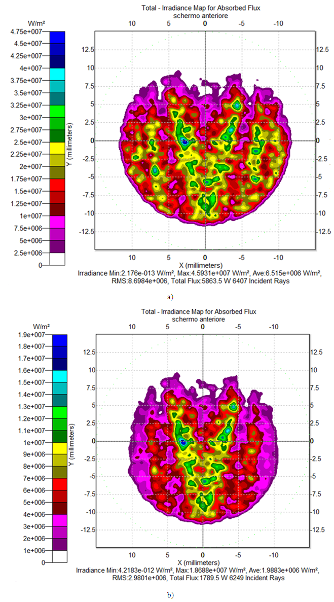
Fig. 18a shows the map of the irradiance obtained on the screen when the wall reflectivity is , whereas Fig. 18b shows the map of the irradiance obtained on the screen when the wall reflectivity is reduced to 0.8. Both simulations were carried out with 2.5M incident rays.

The comparison between Fig. 18a and Fig. 18b shows some interesting aspects. First, we note that the central region, characterized by a V-shape, is only slightly attenuated reducing, because this area refers to the back-reflected rays characterized by a low number of reflections on the inner wall of the CPC, around 2 or 3, therefore implying a limited attenuation, of 0.8² = 0.64 or 0.8³ ≈ 0.5. The outermost regions, on the other hand, being crossed by rays that make 5-7 internal reflections, show a stronger attenuation, around 0.3-0.2. But the most interesting comparison is the one between the map of Fig. 14a and that of Fig. 18a. The first concerns the transmitted rays, while the second concerns the reflected rays. Is clear that the two maps should be complementary, and in fact this is what we can see. At the top of the map of Fig. 14a we see a very intense region that, in the map of Fig. 18a, is completely devoid of any ray. The central region with V-shape in Fig. 14a, which is devoid of any ray, in Fig. 18a is the most intense region of the map. And so forth, observing the lateral regions of the two maps, we can see that the most intense regions of one map correspond to the less intense regions in the other map, and vice versa.

We are now able to obtain the map of the number of reflections made by the back-reflected rays, by applying Eq. (8) in which the quantities and correspond to the ones in maps of Figs. 18a and 18b, respectively.

The number of rays and are obtained by the raytracing results. Fig. 19 shows the map of the average number of internal reflections made by the reflected rays. The different areas of the map are distinguished by different colors and labeled with the corresponding number of internal reflections. We first note a marked difference with the map of transmitted rays in Fig. 15, because the average number of reflections made by the reflected rays is higher than the average number of reflections made by the transmitted rays. A discussion about this and further results is reported in next section.

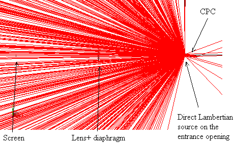Figure 17. Raytracing of the direct irradiation of entrance opening of the CPC by a Lambertian source with 90° divergence. The CPC is oriented at θin= 5° off the z direction, counterclockwise around the x axis

Figure 18. Intensity maps measured on the screen of Fig. 5 when the CPC is oriented at θin= 5° respect to the z axis and the entrance opening is irradiated in direct mode by a Lambertian beam with 10° divergence. (a) Wall reflectivity Rw = 1.0; (b) wall reflectivity Rw = 0.8

5. Discussion

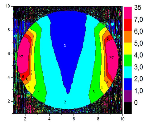
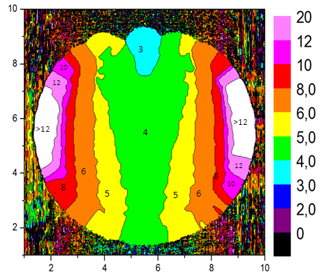
The maps of Fig. 15 and 19 should be complementary, that is, they should show only the regions that are crossed by the transmitted rays or by the reflected rays, respectively. On the contrary, the maps resulting by the two simulations are full, and this makes it difficult to interpret the results. The difficulty arises from the fact that the two intensity maps of (Fig. 14a and 14b) from which we obtained the map of n (Fig. 15) do not have an intensity exactly equal to zero in the regions crossed by the reflected rays, due to the low angular resolution of the simulations. Similarly, the two intensity maps (Fig. 18a and 18b) from which we obtained the map of m (Fig. 19) do not have an intensity exactly equal to zero in the regions crossed by the transmitted rays, also in this case because of the low angular resolution of the simulations. As consequence of this, in the regions in which the intensity should be zero, the simulation program is not prevented to derive, for these regions, a certain value of the number of internal reflections n or m through Eq. (7) or Eq. (8), respectively, even if the intensity is low in both regions.

Therefore, to extract the correct information of n or m from the two maps, it becomes necessary to compare them to the intensity maps and neglect the regions in which the intensity is too low. To do this, we selected from the map of Fig. 15 only the regions that, in the map of Fig. 14a, had the highest intensity and roughly occupied half of the circular area. Operating in the same way, we obtained the map of Fig. 19 by selecting, in the map of Fig. 18a, only those regions that had the highest intensity and roughly occupied half of the circular area. The two maps are in fact spatially complementary and the areas occupied by them must be equal. Combining the two maps, we obtain the map of Fig. 20. In this map, the thicker line separates the regions referred to the transmitted rays from the regions referred to the reflected rays. The regions referred to the transmitted rays are full colored, while those referred to the reflected rays are spray colored. From Fig. 20 we note that the regions referred to the transmitted rays are well defined, that is adjacent regions differing only by one internal reflection are well separated; instead, we notice that the individual regions referred to the reflected rays contain a range, sometimes large, of number of reflections. All this, again, is a consequence of the fact that the angular resolution of the simulations is too low to better distinguish the different regions between them. As consequence, the regions referred to reflected rays, that are in general thinner than those referred to transmitted rays, cannot be well resolved. What the low angular resolution prevents to do is also the separation of the thin bands of n from the thin bands of m, which should alternate within the map and vertically extend in the left and right sides of it, as it is illustrated in the example of Fig. 2.

The map of Fig. 20 is then to be considered as a rather approximate map of the real one. We might get a more reliable map improving the angular resolution of the optical simulations, but this implies increased processing times, well higher than 12 hours, which are not always tolerated by a code running on a personal computer. The alternative would be to transfer these simulations on a more powerful computer. We believe, therefore, that the results achieved so far are the best ones that can be achieved as a first attempt and that they should thus be considered as a first, rough result of the proposed method: the map of the average number of internal reflections made by the transmitted and reflected rays in a 3D-CPC. We refer to a subsequent job research for more reliable results, possibly including more simulations at other tilting angles of the CPC.

Figure 19. Map of the entrance aperture describing the distribution of number of reflections made on the internal wall by incident rays at 5° on the CPC before being back-reflected through the entrance opening

Figure 20. A tentative map of the entrance aperture describing the combined distribution of number of reflections made on the internal wall by rays incident at 5° on the CPC before being transmitted and of number of reflections made on the internal wall by incident rays at 5° on the CPC before being back-reflected. The thicker line separates the transmitted and reflected rays regions. The regions of interest to the transmitted rays are full colored, while those referring to the reflected rays are spray colored

6. Conclusions

In conclusion, in this work we have presented the results of new optical simulations performed on a 3D-CPC nonimaging concentrator, irradiated in direct mode by a parallel beam. This simulation work is the fourth of a series, and the third one discussing the practical applications of the theoretical methods presented in this series. In this work, we have analyzed the optical properties of a 3D-CPC with canonical shape (no truncation), with an acceptance angle at collimated light of 5° and maximum exit angle of 90° at 5° incidence. The CPC has been analyzed by using a ray-tracing program. We have explored its transmission and reflection properties in terms of average number of internal reflections made by both the transmitted and the reflected rays. This study is interesting because it helps to understand the secret mechanisms of light concentration in a 3D-CPC, even if generally of less practical importance. In a previous work of this series, we have analyzed almost all the optical properties of the 3D-CPC irradiated by a collimated beam, oriented at different polar angles with respect to the optical axis. In the present work, we have focused our attention on the number of internal reflections that the incident rays experience before being transmitted or reflected. We have analyzed these aspects by irradiating the CPC just at two incident angles of particularly practical importance: at 0°, that is at the operating angle of the solar concentrator, and at the acceptance angle of 5°, that establishes the limiting operating conditions of the CPC. In the end, we got the summary maps, among which the one at 0° is quite accurate, while the one obtained at the acceptance angle is quite rough, but it gives an idea of what happens to the incident rays. A further work at higher resolution might produce more accurate maps of the number of internal reflections, and thus should be highly desirable, together with maps at other incidence angles.