R. Rhanim1, Y. Tounsi1, A. Ghlaifan1, H. Rhanim2, A. Nassim1
1Laboratory of Measurement and Control Instrumentation IMC, Physics Department, Chouaib Doukkali University, El Jadida, Morocco
2Laboratory of Mechanics and Energetic LME, Physics Department, Chouaib Doukkali University, El Jadida, Morocco
Correspondence to: A. Nassim, Laboratory of Measurement and Control Instrumentation IMC, Physics Department, Chouaib Doukkali University, El Jadida, Morocco.
| Email: |  |
Copyright © 2016 Scientific & Academic Publishing. All Rights Reserved.
This work is licensed under the Creative Commons Attribution International License (CC BY).
http://creativecommons.org/licenses/by/4.0/

Abstract
This work concerns the study of stresses distribution in a photoelastic specimen by using bi-dimensional Photoelasticimetry and optical phase evaluation methods. In Photoelasticimetry technique, isochromatic fringe patterns are generated experimentally by a circular polariscope and the phase distribution is extracted from the monogenic signal. The monogenic signal that is an extension of the analytic signal is obtained by Riesz transform. Finally, the principal stress distributions are determined from the optical phase distribution. In this work, the experimental results are compared to numerical finite element study.
Keywords:
Bi-dimensional Photoelasticimetry, Circular polariscope, Isochromatic fringes, Stress distribution, Monogenic signal, Phase extraction, Finite element
Cite this paper: R. Rhanim, Y. Tounsi, A. Ghlaifan, H. Rhanim, A. Nassim, A Monogenic Phase Extraction Method Applied in Photoelasticimetric Technique for Principal Stress Distribution Determination, International Journal of Optics and Applications, Vol. 6 No. 1, 2016, pp. 7-12. doi: 10.5923/j.optics.20160601.02.
1. Introduction
Bidimensional Photoelasticimetry is an experimental technique based on an optomechanical property called birefringence, which directly provides the whole-field information of principal stress difference and principal stress direction in a specimen. It has a wide range of industrial and research applications [1]. Recent advances of digital Photoelasticimetry have made the analysis of two- dimensional problems faster, accurate and reliable [2, 3]. Recently several methods of analyzing Photoelasticimetric fringe patterns by means of phase evaluation techniques have been presented [4, 5]. There are many methods to extract optical phase’s distribution from fringe patterns such as Fourier-transform method [6] Wavelets methods [7, 8], and monogenic signal [9].Photoelasticimetry has been used as a useful tool for validating finite element analysis for many problems [10, 11]. Researchers have used stress separation method to determine the individual stress components from Photoelasticimetric analysis and then compared them with those obtained from a finite element (FE) analysis. Since FE analysis can provide the stress components easily, methods to post process the FE results to plot Photoelasticimetric contours to compare with experimental results have been reported on a two-dimensional model and stress-frozen slice [12].In this paper, phase evaluation method based on monogenic signal is developed to extract principal stress distribution. The result from Photoelasticimetric experiment was compared to show the usefulness of the finite element simulation (FE plotting scheme). Detailed finite element procedure will be presented and discussed.This work is presented in four sections; the first present the photoelasticimetry technique and the experimental setup used in this technique as well as we detailed the Jones formalism. The second section is a presentation of the Riesz transform and monogenic signal, the third present a detailed finite element procedure and we finish by presenting our results.
2. Photoelasticimetry technique
2.1. Circular Polariscope
The polariscope is an optical system [13, 14] that utilizes the properties of polarized light in its operation, as shown in figure 1, it consists of a light source, an analyzer  polarizer P, two-quarter-wave plates Q and stressed transparent model (specimen) R. In the same figure, Pθ where θ=90° indicates the polarizer whose transmission axis is perpendicular to the chosen x-axis. Qβ where β=45° indicates the first quarter-wave plate with fast axis at 45°.
  stands for the stressed photoelastic specimen taken as a retardation
  and whose fast axis is at an angle
  with the x-axis.
  indicates the second quarter-wave plate with fast axis at
 indicates the analyzer whose transmission axis is
  to the chosen x-axis.
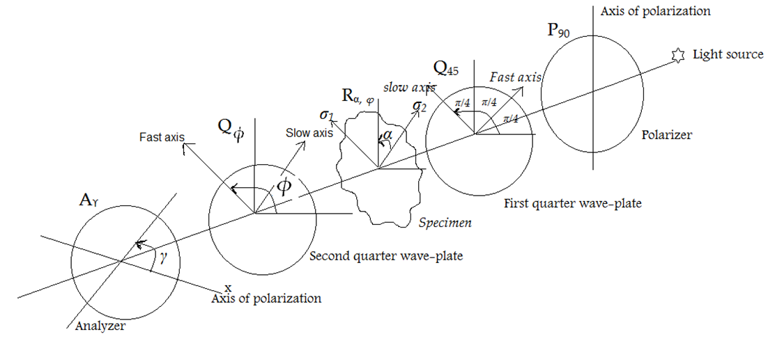 | Figure 1. Optical arrangement of a circular polariscope |
In Jones representation [15], each optical element is represented by a Jones matrix and the polarized light is represented by Jones’s vector. We denote M1, M2, M3, M4 and M5 respectively the Jones’s matrix of a polarizer, first quarter wave-plate, stressed transparent model, second quarter wave-plate, and analyzer. 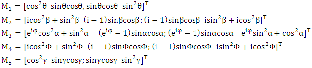 With the Jones calculus, the electric field components are given as:
  | (1) |
Where ω is the angular frequency of light and K is a proportional constant. When the polarized light passed through the stressed transparent model, an interference pattern on fringes is formed. The pattern provides qualitative information about the general distribution of stress, position of stress concentrations and areas of load stress.From the two components, we obtain the intensity distribution of these fringe patterns formed as: | (2) |
Where  and
and  are the complex conjugates of electric field components. For the arrangement of
 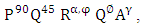 the matrix M1 and M2 become:
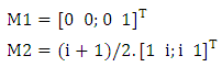 And the output light intensity is given as:
 | (3) |
It’s the intensity distribution of isoclinic fringes encoded in angle α and isochromatic fringes encoded in angle φ, these fringe patterns provide respectively the principal stress directions and the principal stress differences [16]. Isoclinic fringes depend on the orientation of crossed filter set whereas the isochromatic fringes depend on the stress-optic effect.
2.2. Isochromatic Fringes
The main problem of photoelasticimetry technique is that isoclinic and isochromatic fringes pattern are completely mixed, so we can’t analyze them simultaneously, for this reason, the compressed specimen is placed in a circular polariscope. The Circular Polariscope configuration is used for determining the magnitude of principal stress difference. We choose the circular configuration  in which the polarizer/analyzer pairs are then rotated as a unit until their axes are aligned with the birefringent indicial axes, and the quarter- wave plates are then reinserted with their axes oriented at the usual 45° angle with respect to the new polarizer axes. The system is now in the standard circular dark-field polariscope condition. Up to this point the polarizer/analyzer axes have been kept orthogonal to each other, but now the analyzer is rotated separately until one of the fringes moves over the selected point. In rotating the analyzer up to 90°, the polariscope is changing from a dark-field. According to the Jones calculus, the intensity distribution in this case (the circular configuration) becomes:
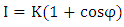 | (4) |
The optical phase distribution is related to the path difference or retardation  by:
by: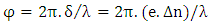 | (5) |
The physical origin of the retardation  is the stress-induced optical anisotropy of the specimen. As well as the birefringence is related to principal stress difference by:
 | (6) |
From (5) and (6), the phase is expressed as: 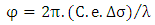 | (7) |
Where  is the wavelength of light;
  is the optical path difference; e is the thickness of the specimen, ∆n is the refractive index,
  the principal stress difference and C is the photoelastic constant which characterizes specimen.Owing to the linear relationship between
  and
and  according to equation (7), the principal stress difference may be made automatically from the fringe pattern phase distribution using the monogenic signal that is the aim of next section.
3. Riesz Transform
3.1. Presentation
In signal processing application, the analytic representation of a real value function defined as the linear combination of the original function and its Hilbert transform [17, 18] is a useful tool from which the phase, energy, and instantaneous frequency of a one-dimensional signal may be estimated. The principal challenge is how to generalize this theory for two-dimensional signals. There are several approaches to generalize Hilbert transform to higher dimensions [19, 20], Riesz transform is among these approaches, and it is the natural multidimensional extension of Hilbert transform [21]. For fringe pattern f (two-dimensional signals), the Riesz transform in spatial representation is expressed as: | (8) |
With  stand for the convolution,
  and
and  are the kernels of Riesz defined in spatial representation as:
 | (9) |
3.2. Phase Distribution of Monogenic Signal
The monogenic signal introduced by Sommer and Felsberg is a multi-dimensional isotropic generalization of the 1D analytic signal. It is defined as the combination of two-dimensional signal and its Riesz components. | (10) |
 | (11) |
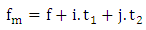
Where i and j are two distinct orthogonal hypercomplex imaginary units. The functions  are the two Riesz components of fringe. In other words, as shown in figure 2, the monogenic is three-dimensional vectors in Cartesian coordinate system
  We can present
  in the spherical coordinate system illustrated in the same figure, from this representation, several features can be extracted (amplitude, local orientation, and local phase), this tree features are orthogonal, that means that represent an independent information.
  | Figure 2. Geometric illustration of the monogenic signal in a spherical coordinate system |
The local amplitude that represents the local intensity or dynamics is defined by: | (12) |
The Local phase represents the structural information; it denotes the angle between amplitude and the plane spanned by the two complex vectors.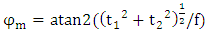 | (13) |
The local orientation represents the geometrical information meaning the direction of phase information. | (14) |
A fourth feature can be defined phase vector, it is a local phase oriented in the vector  such as:
 | (15) |
Several applications of monogenic signal analysis have realized, we cite some paper like temperature measure [22], wavelet filtering [23], and medical imaging [24].
4. Results of Principal Stress Difference
4.1. Photoelasticimetric Study
The experimental data were acquired by a digital camera using a circular polariscope. In this experience, we used a transparent photoelastic polymer. The material of the test specimen is a transparent polymer we have defined as an elastic material whose mechanical properties are Young’s modulus of E=2.7N/mm2 and Poisson ratio of ν=0.48. From one isochromatic fringe pattern (size 636*1332 pixels) and after a post-treatment step of acquired, we obtain isochromatic fringes in grayscale (figure 3.a), from there, we extract the phase distribution presented in figure (3.b) by using monogenic signal. The extracted phase is wrapped or discontinuous because of use of tangent, the unwrapping step is necessary in order to eliminate this discontinuity and get the continuous phase distribution consequently the continuous information as shown in figure (3.c), we used PUMA algorithm [25] for phase unwrapping. The black circular area that we notice in figure (3.a) and figure (3.b) corresponds to the hole in the photoelastic specimen. | Figure 3. (a) Isochromatic fringe pattern (gray scale), (b) wrapped phase distribution obtained using the monogenic signal, (c) continuous phase distribution |
From the two-dimensional phase distribution presented, we plot the gray scale values or intensity variation in terms of distance in pixels as presented in figure 4. We notice that the gray value variation is symmetric in the vicinity of hole.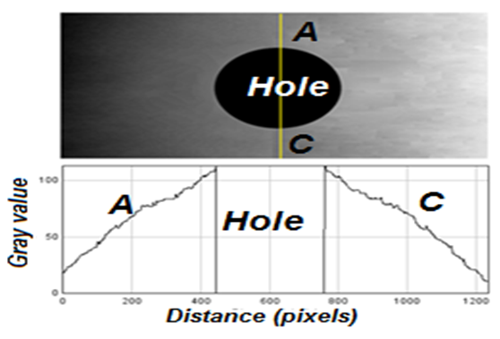 | Figure 4. Intensity distribution along the path in continuous phase distribution |
4.2. Finite Elements Study
Considering the mechanical structure applied to a tensile loading, to be model numerically in order to determine the stress distribution. In figure 5, we present the model study in the form of the specimen used in experience.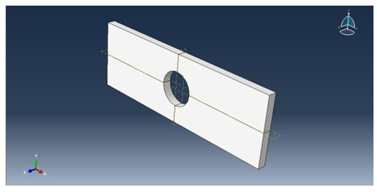 | Figure 5. Model study |
The numerical simulation was made by a numerical computation code. Figure 6 illustrates the specimen that has meshed with quadratic elements of type C3D20R with a total number of elements equal to 2272. A mesh refinement is also established in the vicinity of the defect (hole) to determine the concentration of local stresses and give more precision about the results obtained. 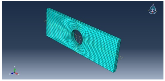 | Figure 6. Meshed specimen |
The material of the test specimen is a transparent polymer we have defined as an elastic material whose mechanical properties are Young’s modulus of E=2.7N/mm2 and Poisson ratio of ν=0.48.The results shown in figure 7 show the distribution of stresses in the specimen breakthrough and urged to tensile loading. It is clear that the load applied to the structure has generated maximum stresses in the vicinity of the hole. Figure (7.c) illustrates the stress distribution along predefined yellow path.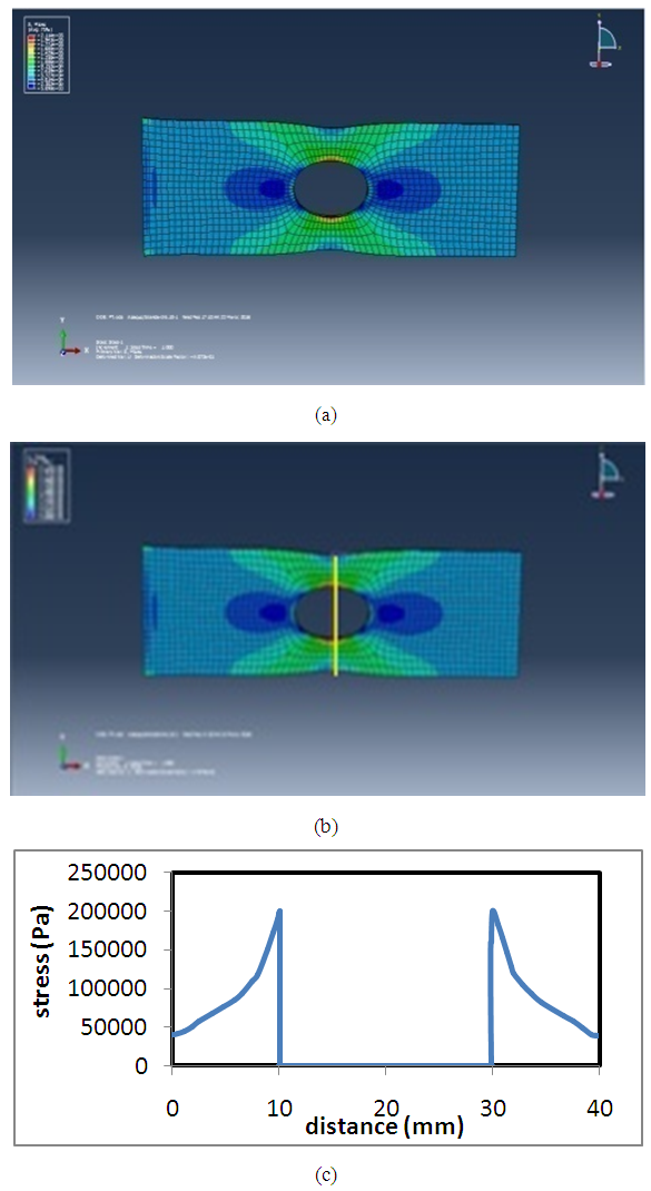 | Figure 7. (a, b) Stresses distribution at the structure along the yellow path (c) stress distribution along the predefined path |
Note that the distribution of the equivalent stress in the specimen mark a maximum stresses concentration in the vicinity of the defect (hole), while away from defect there are low-stress values. Far from the discontinuity specimen is relaxed.
5. Conclusions
We have presented a study based on Photoelasticimetry and optical phase evaluation techniques in order to obtain the stresses distribution in a photoelastic specimen. Especially, we exploited the phase distribution of the isochromatic fringes extracted by monogenic signal to obtain principal stresses distribution. Also, we presented a numerical finite element model and extract the stresses distribution variation along the path indicated in fig (7.a). As it shows results, the two schema plots (fig 6 and fig (7.a) has the same appearance, considering stresses encoded in gray values. It is, therefore, possible to calculate rapidly and accurately stresses and Photoelasticimetry can be successfully used to validate the numerical approach.
References
| [1] | Frocht M. M. Photoelasticity. The Selected Scientific Papers of M. M. Frocht, 1st edition. Oxford, New York: Pergamon, 1969. |
| [2] | Chen T. Y. Digital Photoelasticity in Photomechanics, D. P. K. Rastogi, Éd. Springer Berlin Heidelberg, 2000, p. 197‑232. |
| [3] | Pathak P. M. and Ramesh K. Validation of finite element modeling through photoelastic fringe contours. Communications in Numerical Methods in Engineering, vol. 15, no 4, avr 1999, p. 229‑238. |
| [4] | Buckberry C. and Towers D. Automatic analysis of isochromatic and isoclinic fringes in photoelasticity using phase measuring techniques. Meas. Sci. Technol., vol. 6, no 9, 1995, p. 1227. |
| [5] | Asundi A. Phase Shifting in Photoelasticity. Experimental Techniques, vol. 17, no 1, janv. 1993, p. 19‑23. |
| [6] | Takeda M, Ina H. and Kobayashi S. Fourier-transform method of fringe-pattern analysis for computer-based topography and interferometry. J. Opt. Soc. Am., JOSA, vol. 72, no 1, janv. 1982, p. 156‑160. |
| [7] | Afifi M, Fassi-Fihri A, Marjane M, Nassim K, Sidki M, and Rachafi S. Paul wavelet-based algorithm for optical phase distribution evaluation. Optics Communications, vol. 211, no 1‑6, oct. 2002, p. 47‑51. |
| [8] | Dembele V, Assid K, Alaoui F, Nassim A. K. Squeezed Carrier Interferogram for Wavelet Phase Recovery. International Journal of Optics and Applications, vol. 2, no 4, 2012, p. 38‑42. |
| [9] | Felsberg M and Sommer. The monogenic signal. Signal Processing, IEEE Transactions on, vol. 49, no 12, déc. 2001, p. 3136‑3144. |
| [10] | Sanford R. J. and Beaubien L. A. Stress analysis of a complex part: Photoelasticity vs. finite elements. Experimental Mechanics, vol. 17, no 12, 1977, p. 441‑448. |
| [11] | Guagliano M. and Vergani L. Experimental and numerical analysis of sub-surface cracks in railway wheels. Engineering Fracture Mechanics, vol. 72, no 2, janv. 2005, p. 255‑269, |
| [12] | Babu K. P. R. D, and Ramesh K. Development of photoelastic fringe plotting scheme from 3D FE results. Communications in Numerical Methods in Engineering, vol. 22, no 7, juill. 2006, p. 809‑821. |
| [13] | Dally W. and Riley W. F. Experimental stress analysis. 2nd Ed., McGraw-Hill Inc., (1991). |
| [14] | Cloud G. L. Optical Methods of Engineering Analysis. Revised ed. edition. Cambridge University Press, 1998. |
| [15] | Theocaris P. E. and Gdoutos E. Matrix Theory of Photoelasticity. Springer-Verlag, (1979). |
| [16] | Asundi A, Tong L, and Boay C. G. Determination of isoclinic and isochromatic parameters using the three-load method. Meas. Sci. Technol., vol. 11, no 5, mai 2000, p. 532. |
| [17] | Franks L. E. Signal theory. Engelwood Cliffs: Prentice Hall. 1968. |
| [18] | Gabor D. Theory of communication. Journal of the Institution of Electrical Engineers - Part I: General, vol. 94, no 73, ‑, janv. 1947, p. 58. |
| [19] | Bulow T. Hypercomplex Spectral Signal Representations for the Processing and Analysis of images. ResearchGate, sept. 1999. |
| [20] | Calderon A. P. and Zygmund A. On the existence of certain singular integrals. Acta Math., vol. 88, no 1, 1952,p. 85‑139. |
| [21] | Stein E. and Weiss G. Introduction to Fourier Analysis on Euclidean Spaces. Princeton, NJ: Princeton Univ. Press, 1971. |
| [22] | Zada S, Darfi S, Dembele V, Rachafi S, et A Nassim. Temperature Measurement Method Based on Riesz Transform Method. Int. Sch. Res. Not., vol. 2013, déc. 2013. |
| [23] | Chenouard N. and Unser M. 3D steerable wavelets and monogenic analysis for bioimaging. IEEE International Symposium on Biomedical Imaging: From Nano to Macro, 2011, p. 2132‑2135. |
| [24] | Alessandrini M, Basarab A, Liebgott H., and Bernard O. Myocardial Motion Estimation from Medical Images Using the Monogenic Signal. IEEE Transactions on Image Processing, vol. 22, no 3, mars 2013, p. 1084‑1095. |
| [25] | Bioucas-Dias J. M. and Valadão G. Phase Unwrapping via Graph Cuts. Image Processing, IEEE Transactions on, vol. 16, no 3, mars 2007, p. 698‑709. |

 Abstract
 Reference
 Full-Text PDF
 Full-text HTML