-
Paper Information
- Paper Submission
-
Journal Information
- About This Journal
- Editorial Board
- Current Issue
- Archive
- Author Guidelines
- Contact Us
International Journal of Optics and Applications
p-ISSN: 2168-5053 e-ISSN: 2168-5061
2015; 5(3): 82-102
doi:10.5923/j.optics.20150503.05
Optics of Solar Concentrators. Part III: Models of Light Collection of 3D-CPCs under Direct and Lambertian Irradiation
 Abstract
 Reference
 Full-Text PDF
 Full-text HTML
Antonio Parretta1, 2, Erica Cavallari2
1ENEA C.R. “E. Clementel”, Via Martiri di Monte Sole 4, Bologna (BO), Italy
2Physics Department, University of Ferrara, Via Saragat 1, Ferrara (FE), Italy
Correspondence to: Antonio Parretta, ENEA C.R. “E. Clementel”, Via Martiri di Monte Sole 4, Bologna (BO), Italy.
| Email: |  |
Copyright © 2015 Scientific & Academic Publishing. All Rights Reserved.
The optical properties of nonimaging solar concentrators irradiated in direct mode by diffused Lambertian beams are investigated in detail adopting original simulation methods. These methods were not limited to investigate useful properties for the practical application of the concentrators, but were also used to study them as optical elements with specific transmission, reflection and absorption characteristics. We have investigated, therefore, besides the flux transmitted to the receiver, also the flux back reflected from input aperture and that absorbed on the wall of the concentrator. We have simulated the transmission, reflection and absorption efficiencies, the average number of reflections of the transmitted or reflected rays, their angular divergence and the distribution of flux on the receiver and on the internal wall surface, as function of the angular divergence of the input beam and of the reflectivity of the internal wall. The presented simulation methods can be fruitfully applied to any other type of solar concentrator.
Keywords: Solar concentrator, Light collection, Optical simulation, Optical modeling, Nonimaging optics
Cite this paper: Antonio Parretta, Erica Cavallari, Optics of Solar Concentrators. Part III: Models of Light Collection of 3D-CPCs under Direct and Lambertian Irradiation, International Journal of Optics and Applications, Vol. 5 No. 3, 2015, pp. 82-102. doi: 10.5923/j.optics.20150503.05.
Article Outline
1. Introduction
- A review of the theoretical models of light irradiation and collection in solar concentrators (SC) was presented in the first part of this work [1]. In the second part [2] we presented the optical simulations of those models applied to nonimaging SC irradiated by direct and collimated beams. The importance of this irradiation lies in the fact that it represents the typical operating condition of a SC. We have chosen, for the optical simulations, a class of nonimaging SC of the type 3D-CPC (Three-Dimensional Compound Parabolic Concentrators) [3-9] to be used mainly as primary elements of a concentrator system. In this paper we extend the study of these SC by investigating diffused irradiation conditions, which are well represented by lambertian beams (beams with constant radiance) with variable angular aperture. The results of our work can be extended in this way to CPC used as secondary elements of concentration. Our interest on these SC is that they allow to reach very high concentration levels, comparable to the theoretical ones, and that their optical transmission efficiency is quite constant within a defined angle of incidence of the input beam. A further advantage of these SC is that they operate with reflective surfaces that do not induce spectral dispersion of light. We have simulated the optical behavior of the nonimaging SC by investigating its transmission, reflection and absorption properties, and we have defined new optical quantities. In particular, we have examined: i) the transmitted flux in terms of the optical transmission efficiency, average number of internal reflections of the transmitted rays, spatial distribution of the flux density on the receiver, angular distribution of radiance at the exit aperture; ii) the flux reflected from the input aperture in terms of reflection efficiency, angular divergence and average number of reflections; iii) the absorbed flux in terms of absorption efficiency and distribution of the absorbed flux on the internal wall of the CPC. In this way, all the optical features of the SC, considered as a generic optical element interacting with a lambertian beam, were analyzed. The methods of simulation and elaboration of the optical data presented in this work can be considered as general tools for the analysis of any other optical device.
2. The Compound Parabolic Concentrator (CPC)
- The Compound Parabolic Concentrator (CPC) is a nonimaging concentrator developed by R. Winston [3] to efficiently collect Cherenkov radiation in high energy experiments. Since then, the nonimaging concentrators have been widely used to concentrate sunlight [4-18]. The CPC is a reflective concentrator with a profile obtained by the combination of two parabolas, and is characterized by a step-like transmission efficiency allowing the efficient collection of light from 0° to a maximum angle, the acceptance angle
 , where the suffix “coll” means that the irradiation is done with a collimated beam.Fig. 1 shows the 3D-CPC used in this work for the optical simulations. It is the same that was used in the previous paper of this series [2]. It is characterized by a maximum divergence of rays at exit aperture equal to 90°, and then only two independent parameters are required for defining its shape.
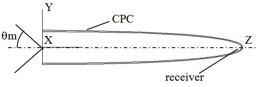 | Figure 1. Longitudinal section of the Compound Parabolic Concentrator (CPC) used in this work for the optical simulations. The angle  is the maximum angle of aperture of the input Lambertian beam. The angle of acceptance of a parallel beam is is the maximum angle of aperture of the input Lambertian beam. The angle of acceptance of a parallel beam is  |
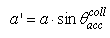
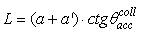
 and the length L = 150 mm. The focal length of the parabolic profile, f = 1.14 mm, the radius of input aperture, a = 12.035 mm, and the radius of output aperture, a’ = 1.052 mm, become [2]:
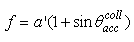 | (1) |
 | (2) |
 | (3) |
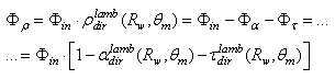
 all the other added devices (absorbers, screens, etc.) were external to the concentrator and were used only as tools to improve the knowledge of its optical properties. For the reflectivity of the internal wall we have used only high values (0.8÷1.0); when not specified, it is equal to 1 (no optical loss inside the concentrator). All the optical simulations were carried out by using the TracePro ray-tracing software of Lambda Research [19].The flux at input of the CPC is a Lambertian flux characterized by a constant radiance
  and by a variable angular aperture
  The total flux at input is then a function of
  and is expressed by [1]:
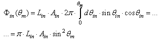 | (4) |
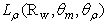
 is the incident polar angle. In order to keep constant the radiance at input of the CPC, we have used in the simulations a number of input rays, that is an input flux, proportional to
3. Analysis of the Transmitted Flux
3.1. Analysis of the Total Flux Transmitted to Receiver
- To study the flux transmitted to the exit aperture of the CPC, we have closed the exit aperture by an ideal absorber, so all the rays reaching the aperture can be counted and analyzed by the simulation program [19]. The flux transmitted to the exit aperture is given by:
 | (5) |
 is the transmission efficiency of the CPC under direct and collimated irradiation, and is a function of the incident polar angle
  [1, 2] (see Fig.2).
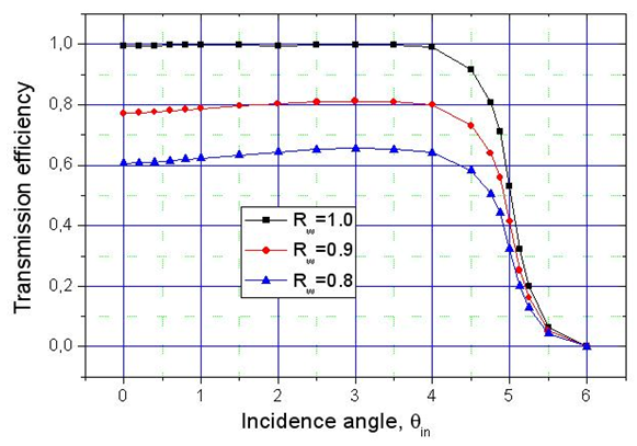 | Figure 2. Optical transmission efficiency  of the 3D-CPC calculated for three wall reflectivities: of the 3D-CPC calculated for three wall reflectivities:  |
 rule (see Eq. (4)), corresponding, in this simulation, to 50k rays at
  Fig. 3 shows the number of the incident, transmitted and reflected rays vs.
  measured for a unitary wall reflectivity. In this case we have no optical loss on the wall of the CPC, but only loss due to the back reflected rays. We can see that, as long as
  due to the square shape of the transmission efficiency of the CPC (see Fig. 2), all the input rays are transmitted, whereas, at
  the transmitted rays stop growing and the reflected rays begin to appear and grow following the growth of the incident rays.
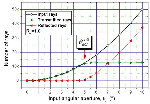 | Figure 3. Number of incident, transmitted and reflected rays vs. the angular aperture of the Lambertian beam  calculated for a unitary wall reflectivity calculated for a unitary wall reflectivity |
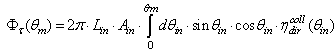
 [1].This quantity refers to an angular aperture of the Lambertian beam equal to 90°. If the lambertian beam at input is limited by the angular aperture
  the above quantity becomes
  We have added the term "dir" to distinguish the Lambertian beam that we send to the entrance aperture of the concentrator, from the Lambertian beam that we send to the exit aperture of the concentrator, and that we will indicate by the term "inv". The properties of a CPC concentrator irradiated by an “inverse” Lambertian beam will be discussed in a future paper of this series. The Lambertian transmission efficiency of the CPC is expressed [1] by the ratio between output and input flux:
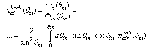 | (6) |
 simulated for a unitary wall reflectivity, is shown in Fig. 4. It is interesting to compare the behavior of
  with that of
  (see Fig.2). We obtain a step-like transmission efficiency curve also for a Lambertian beam irradiation, with the efficiency almost constant until about the acceptance angle
  but, differently from the transmission efficiency curve
  now the
  curve decreases slowly at increasing
  The reason is that, for
  a constant portion of the input beam is always collected, and the Lambertian transmission efficiency at these conditions can be expressed by (on the assumption that
  =1.0):
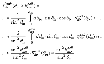 | (7) |
 as it can be seen from the curve of Fig. 2 corresponding to
  Fig. 4 shows the Lambertian transmission efficiency of the CPC compared to the
 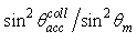 function. The perfect correspondence between the two curves when
  is clearly evident.
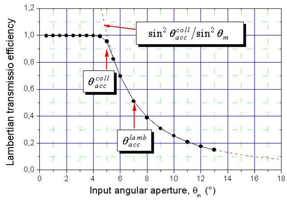 | Figure 4. Lambertian transmission efficiency of the CPC calculated as function of the angular aperture of the Lambertian beam,  for a unitary wall reflectivity for a unitary wall reflectivity |
 We call this angle the “Lambertian acceptance angle”,
  indicated in Fig. 4 together with
  the acceptance angle at parallel beam irradiation. The quantity
  is immediately derived from Eq. (7), and is about 7.1° for our CPC with
  = 5.0°:
 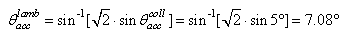 | (8) |
 Until now we have not yet analyzed the effect of
  on the studied quantities. We do it starting with the direct Lambertian transmittance, calculated for three wall reflectivities:
  =1.0, 0.9 and 0.8 (see Fig. 5).
 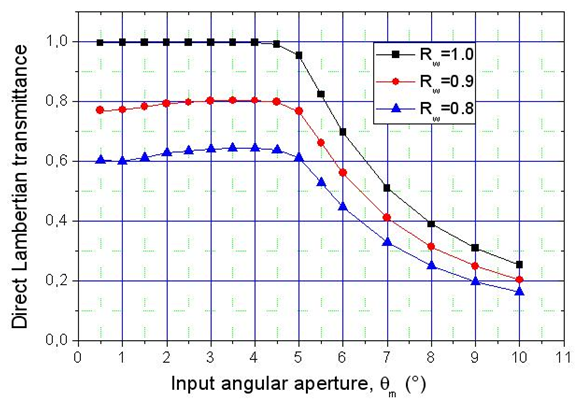 | Figure 5. The Lambertian transmission efficiency calculated for three different wall reflectivities:  =1.0; 0.9 and 0.8 =1.0; 0.9 and 0.8 |
3.2. Average Number of Reflections of the Total Absorbed Rays
- The analysis of the three curves of
 allows deriving the average number of reflections experienced by the transmitted rays. In this regard we will make use of a formula similar to Eq. (24) used in [2], replacing
  with
with 
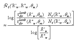 | (9) |
 represents the number of transmitted rays. The average number of reflections has been calculated by using three pairs of wall reflectivities: (1.0-0.9); (1.0-0.8); (0.9-0.8). The results are reported in Fig. 6 and show that the average number of reflections of the transmitted rays is practically independent on the angular aperture of the Lambertian beam and equal to ≈2. This result is in good agreement with what was found [2] by analyzing the average number of reflections of the transmitted beam when the CPC is irradiated with a parallel beam at different polar angles respect to the optical axis.
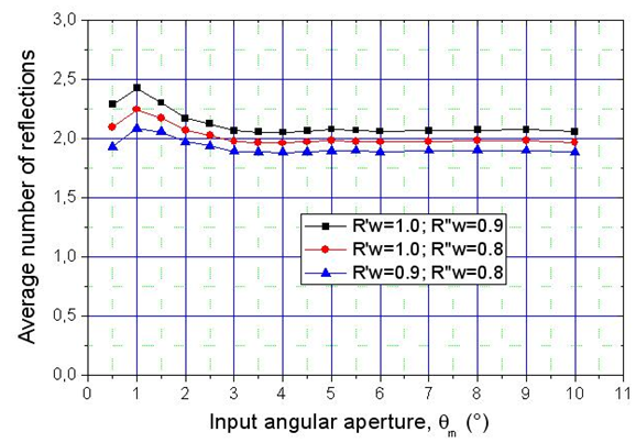 | Figure 6. Average number of reflections experienced by the transmitted rays, as function of the angular aperture of the Lambertian beam, calculated for three pairs of wall reflectivities: (1.0-0.9); (1.0-0.8); (0.9-0.8) |
3.3. Lambertian Concentration Ratio
- We now introduce the quantity “direct Lambertian concentration ratio”,
 defined in [1] as the ratio between the average output, or transmitted, radiance and the constant input radiance. When the lambertian beam at input has an angular aperture
  the direct Lambertian concentration ratio is indicated as
  We start calculating the average output radiance:
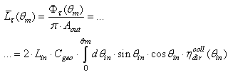 | (10) |
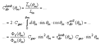 | (11) |
 expressed in (W/mm2·sr) and calculated for three wall reflectivities:
  =1.0, 0.9 and 0.8.
 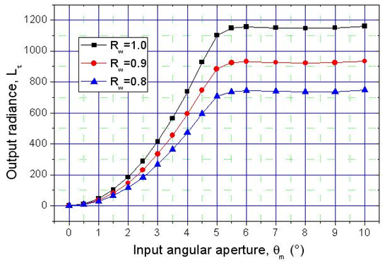 | Figure 7. Average output radiance  of the transmitted flux, calculated for three wall reflectivities: 1.0, 0.9 and 0.8 of the transmitted flux, calculated for three wall reflectivities: 1.0, 0.9 and 0.8 |
 calculated from Eq. (11) is reported in Fig. 8.
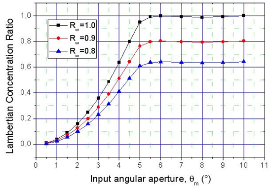 | Figure 8. Direct lambertian concentration ratio,  calculated for three wall reflectivities: calculated for three wall reflectivities:  = 1.0, 0.9 and 0.8 = 1.0, 0.9 and 0.8 |
 is always ≤1, that is the average output radiance is always smaller than the input radiance, being equal to it only when the internal wall is an ideal mirror and the input angular aperture is greater than the acceptance angle of the CPC (5°). This can be easily demonstrated considering that, for
  we have:
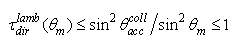 | (12) |

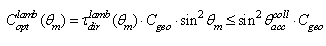
 (11’)Considering that
  corresponds to the maximum value of the optical concentration ratio, equal to
  [1], from Eq. (11’) we conclude that
3.4. Analysis of the Flux Distribution on the Receiver
- To study the flux transmitted to the exit aperture of the CPC, the exit aperture was closed by an ideal absorber. Fig. 9 shows the maps of the irradiance on the receiver as function of the angular aperture of the lambertian beam at input, from 1.0° to 6.0°; the wall reflectivity is 1.0. Contrary to the maps obtained by irradiating the CPC with a parallel beam [2], the maps of Fig. 9 are symmetric respect to the optical axis, as consequence of the rotational symmetry of both the CPC and the lambertian beam. The optical simulations were performed by setting a number of input rays
 =100k for
  then
then  is given by:
 | (13) |
 then it is distributed in the central part
 the center is impoverished, but again, starting from
 we have an almost uniform distribution of the flux in the central part of the receiver, which extends to the edge at increasing
  , to become uniform when
  reaches a value equal to the acceptance angle (5°). Then we can say that the flow affects at first the central part of the receiver and then the outer ring. In essence, the less inclined rays gather in the central part of the receiver, while those more inclined gather on its edge.We can see from Fig. 10a, where the wall reflectivity is unitary and we have no optical losses inside the CPC, that the output irradiance profile becomes flat as soon as the angular aperture
 exceeds the acceptance angle (5.0°). By reducing
  the irradiance profiles are slightly smoothed, because of the optical loss inside the CPC; at the same time, they become blunt at the edges, because the optical loss is higher there as an effect of the higher number of reflections, as we will see shortly after.
 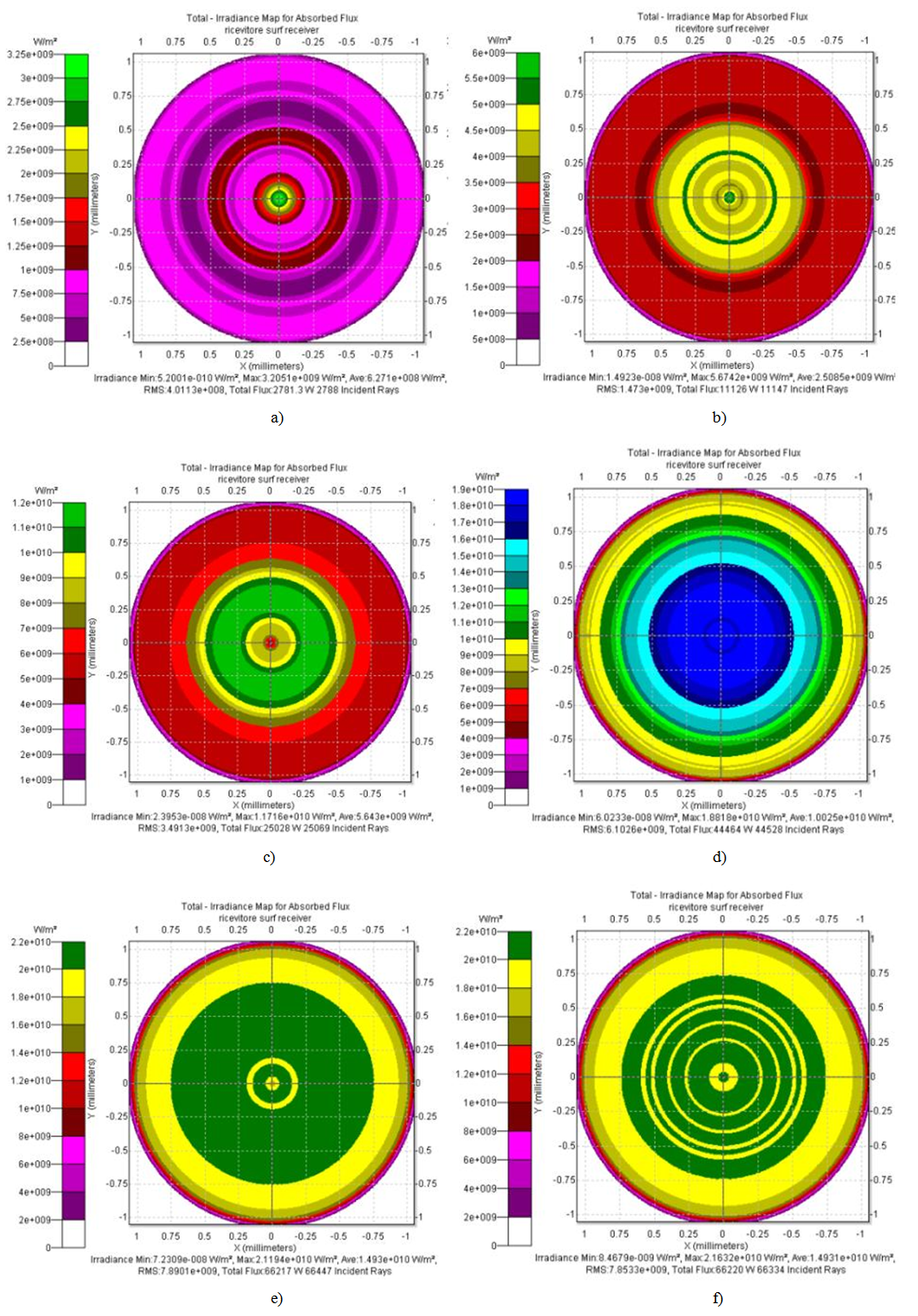 | Figure 9. Maps of output flux on the receiver for different angular apertures of the lambertian beam at input:  = 1.0° (a); 2.0° (b); 3.0° (c); 4.0° (d); 5.0° (e); 6.0° (f). Number of input rays: 100k at = 1.0° (a); 2.0° (b); 3.0° (c); 4.0° (d); 5.0° (e); 6.0° (f). Number of input rays: 100k at  = 6°. = 6°.  = 1.0 = 1.0 |
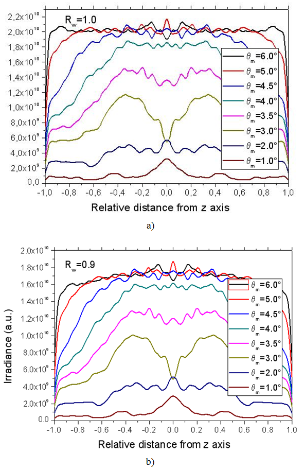 | Figure 10. Irradiance profiles of the flux at output of the CPC, irradiated by a lambertian beam of different angular apertures  Wall reflectivity: Wall reflectivity:  |
3.5. Average Number of Reflections of Locally Absorbed Rays
- As done for the total flux transmitted to the receiver, we are able now to evaluate the average number of reflections experienced by the rays reaching a specific point on the receiver. We use therefore the same Eq. (9), to be applied to the irradiance profiles of transmitted flux, calculated for different values of the wall reflectivity. The irradiance is expressed as:
 where x is the relative distance from the optical axis of the point on the receiver. The average number of reflections
  calculated for a specific value of
  can be therefore obtained from two simulations taken at different wall reflectivities, as follows:
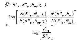 | (14) |
 interval, experience before reaching a point on the receiver. As we are interested to know the average number of reflections done by the rays inclined in a narrow range
  centered at a particular
  value, we have calculated new irradiance profiles,
  obtained as:
 | (15) |
 and from these profiles we have obtained the searched result:
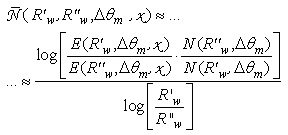 | (16) |
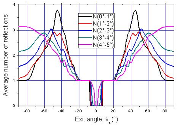
 calculated for the five angular intervals:
 The curves have a very interesting behavior. First of all, they overlap quite well, showing that the number of reflections of rays reaching a specific point at distance x, is only slightly dependent on the angular divergence at input. This is particularly true for middle values of x, less for the points at the center and at the edge of the receiver. The second consideration to do is that
  is low at the center of the receiver, between about 1 and 2, and grows moving towards the edges, reaching values between about 3 and 5. This explains the statement made at the end of section 3.4.As
  is not too much dependent on
  it is interesting to calculate its average respect to the different angular aperture intervals
  . The average quantity
  is shown in Fig. 12 (black curve). It is a very smooth curve, no longer containing the strong oscillations of the curves of Fig. 11.
 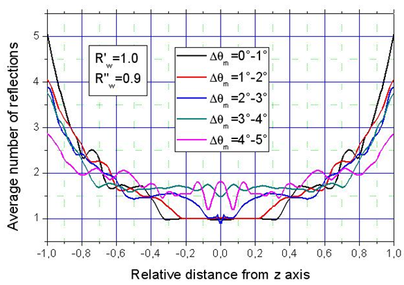 | Figure 11. Average number of reflections of the rays incident at x relative distance from the optical axis on the exit aperture of the 3D-CPC, irradiated by a lambertian beam with different values of angular divergence  |
 is well fitted by the fourth degree polynomial (see red curve in Fig. 12):
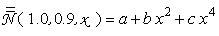 | (17) |
 | Figure 12. Average number of reflections of the rays incident at x distance from the optical axis on the exit aperture of the 3D-CPC, irradiated by a lambertian beam with angular divergence  = 0°-5° (black curve). The red curve is the fitting polynomial = 0°-5° (black curve). The red curve is the fitting polynomial |
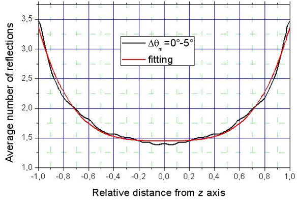
 simulated for an angular aperture of the lambertian beam equal to 1°. The curve shows that
  is exactly 1.0 in the central part of the receiver and increases with a step-like behavior moving towards the edge of the receiver, where the rays arrive after exactly 5 reflections. The rays at input are almost parallel to the optical axis, then the black curve of Fig. 13 is very similar to the red curve obtained in [2] when a collimated beam parallel to the optical axis irradiates the CPC. The difference between the two curves is very little: the red curve has a slightly larger zone with one reflection, and the number of reflections for the rays on the edge is now seven.
 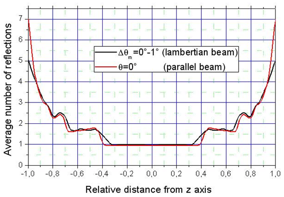 | Figure 13. Average number of reflections of the rays incident on the receiver at x distance from the optical axis. The CPC is irradiated by a lambertian beam with angular divergence  = 0°-1° (black curve) and by a collimated beam parallel to the optical axis of the CPC (red curve) = 0°-1° (black curve) and by a collimated beam parallel to the optical axis of the CPC (red curve) |
3.6. Angular Divergence of the Transmitted Rays
- The study of the angular divergence of rays at output of the CPC is important to optimize the absorption properties of the receiver. In the practical use of a PV solar concentrator, for example, the receiver is not an ideal absorber, but a solar cell with specific reflectance properties, that affect its light absorption capabilities in relation to the divergence of the incoming rays [20]. The flux absorbed by the solar cell can be expressed as:
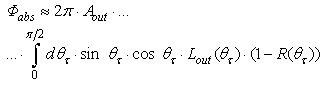 | (18) |
 is the area of the cell,
  is the angle-resolved reflectance and
  is the radiance of light transmitted at exit angle
  by the CPC (the radiance is not function of the azimuthal angle
  because the system input beam + CPC is rotationally symmetric). In Eq. (18), in general
  grows with
  [20], then it is desirable that
  be not too high for high
  values. To check the angular distribution of radiance of light at the CPC receiver, we have irradiated the ideal CPC (
 = 1.0) by a lambertian beam with different values of the angular aperture
  and the output flux has been collected by a hemispherical absorber (radius
  = 200 mm) centered on the receiver (see Fig. 14). The rotationally symmetric map of the flux density on the internal screen surface, projected on a plane orthogonal to the optical axis (see Fig. 16) and the corresponding radial profile, simulated at
  are shown in Fig. 15.
 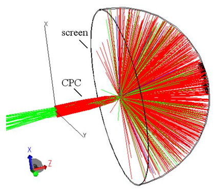 | Figure 14. Scheme of the CPC irradiated by a lambertian beam with 5° angular aperture,  The transmitted rays are collected by a hemispherical screen with a radius The transmitted rays are collected by a hemispherical screen with a radius  Some of rays (green color) are back reflected and attenuated because the wall reflectivity is Some of rays (green color) are back reflected and attenuated because the wall reflectivity is  = 0.9. Most of rays are transmitted and impact on the spherical screen; the red rays are less attenuated (lower number of reflections inside the CPC), whereas the green rays are more attenuated (higher number of reflections inside the CPC) = 0.9. Most of rays are transmitted and impact on the spherical screen; the red rays are less attenuated (lower number of reflections inside the CPC), whereas the green rays are more attenuated (higher number of reflections inside the CPC) |
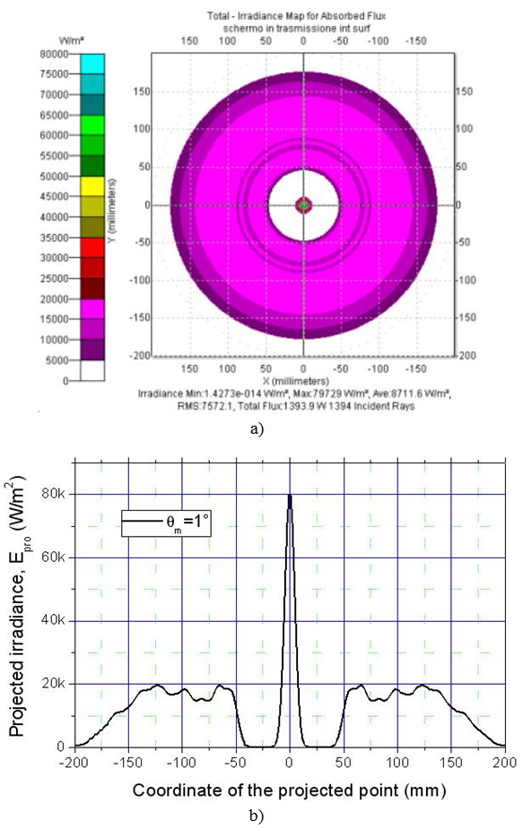 | Figure 15. Map (a) and corresponding radial profile (b) of the flux density (irradiance) (in  ) produced on the screen, projected over a plane orthogonal to the optical axis. The input is a lambertian beam with ) produced on the screen, projected over a plane orthogonal to the optical axis. The input is a lambertian beam with  |
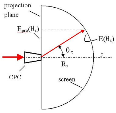 | Figure 16. Schematic representation of the transmission of light to the spherical screen, the production of a flux density (irradiance)  on its internal wall and the projection of this irradiance, on its internal wall and the projection of this irradiance,  on a plane orthogonal to the optical axis on a plane orthogonal to the optical axis |
 (W/m2) is the irradiance on the screen surface,
  (W/m2) is its projection on the orthogonal plane and
  (W/sr) is the radiant intensity, the radiance
  (W/m2sr) of the transmitted light becomes:
 | (19) |
 is the area of the output aperture of the CPC and
  is the screen radius. From Eq. (19) we see that the profile of
  that reported in Fig. 15b, is the same of the radiance
 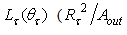 is a constant factor), and then the flux map of Fig. 15 is qualitatively the map of the transmitted radiance. The profile of
  is worth of being analyzed in detail. Fig. 17 shows the effect of the angular divergence
  on the angular distribution of radiance of the transmitted beam, for a wall reflectivity
  = 1.0 (no optical loss by absorption). The number of rays incident at input aperture are a function of
  and follows the
  rule, which, in this case, corresponds to 50k at
  = 6°. The angular divergence
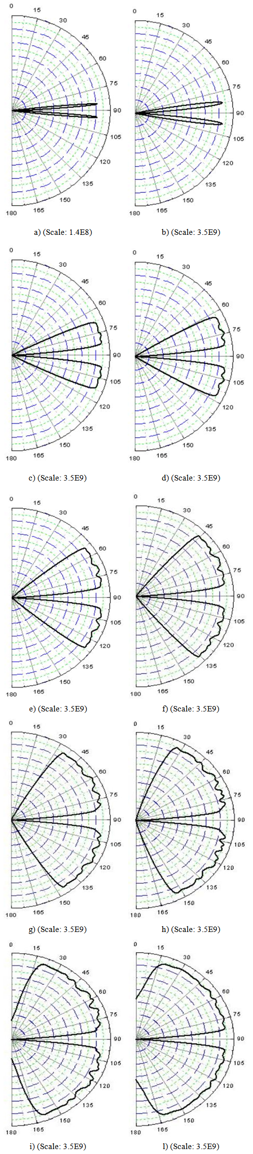
  was varied from 1° to 10° with 1° steps, but we show in Fig. 17 only the first six diagrams, because the polar profiles of
  do not change significantly for
  apart from small fluctuations at near
  The radiance profiles show a strong central peak at
 values. This peak is mainly produced by rays traveling close to the optical axis and crossing undisturbed the CPC without reflections on the internal wall. At
 we find a “dead” zone large ≈ 15°, with no rays, followed by a large band of radiance extending from about 15° to 60°, that takes, near the acceptance angle, the characteristic shape of a “butterfly” or “dragonfly”. The “dead” zone is very similar to that occurring with irradiation by a collimated beam parallel to the optical axis [2]. In that work, we could explain that the dead zone upper limit (about 15°) was due to those rays impacting on the CPC wall at about 7 mm far from the axis, and coming out with a divergence of about 15°; this divergence is a lower limit, since away more from the axis, these rays undergo a second reflection that makes them diverge even more, and therefore makes it impossible exit angles of less than about 15°. Despite being the irradiation Lambertian, instead of parallel, this phenomenon is maintained, because the lambertian beam contains incoming parallel rays parallel or nearly parallel to the optical axis. When the input angular divergence
  reaches the acceptance angle (5°), the radiance profile is quite flat up to 75° (the small fluctuations depend only on the limited number of incident rays) and keeps almost equal up to
  The same profile of transmitted radiance was achieved by increasing
  Fig. 18a shows, for example, the transmitted radiance profile obtained at
  The simulation was carried out with a flux of 400k rays (400k W) and a processing time of about 12 hours; the number of rays, however, was less than would have been necessary to satisfy the
  rule, which assures a constant radiance at input: ~ 4.5M rays and ~130 hours of processing time. The consequence is a loss in the signal-to-noise ratio, as it can be seen in Fig. 18a. Apart from the low signal-to-noise ratio, the simulation at
 has not changed significantly the radiance profile found at 6° (see Fig. 17f) (we know in fact from [2], section 4.2, that input rays tilted more than ≈ 5.8° have no chances to reach the CPC exit opening): a quite flat profile at ~ 3.2·109 W/m2·sr from 0° to 75°, followed by a decay up to ~ 1.6·109 W/m2·sr at 90°. Despite not flat up to 90°, this is effectively the profile obtained with a lambertian beam. This was verified by irradiating the hemispherical screen directly with a lambertian beam, after removing the CPC. The result is the profile of Fig. 18b, where the intensity drops to 50% of maximum at the exit angle of 90°.The evolution of the radiance profiles as function of
  can be followed also transforming the radiance polar diagrams of Fig. 17 into Cartesian diagrams and overlapping them (see Fig. 19). I added also the
  profile obtained at a reduced processing time (~11 times), distinguishable for the low signal-to-noise ratio. Apart from the radiance peak near
  that we have already discussed, we see that the radiance profile monotonically grows in the
  interval at increasing
  from 1° to 4°. A significant change in the radiance profile happens in the
  interval, where we observe the filling of the dead zone at low
  values, as well as of the region between ~20° and ~75°; the 75°-90° interval remains unfilled as explained before.
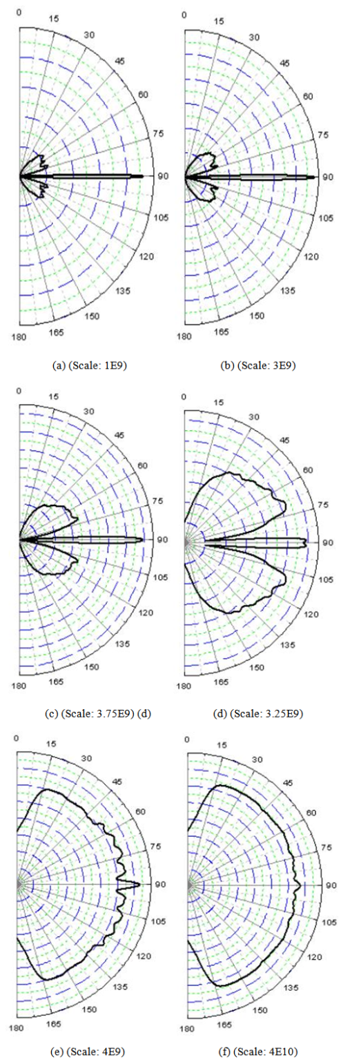 | Figure 17. Polar representation of the distribution of the radiance of the transmitted flux, when the CPC is irradiated with a lambertian beam with angular divergence  = 1° (a); 2° (b); 3° (c); 4° (d); 5° (e); 6° (f). For the angular divergence = 1° (a); 2° (b); 3° (c); 4° (d); 5° (e); 6° (f). For the angular divergence  = 6° (f), We have used 500k rays at input, 10 times more than required to follow the = 6° (f), We have used 500k rays at input, 10 times more than required to follow the   rule. The scale of radiance is expressed in rule. The scale of radiance is expressed in  and is reported near each figure. The wall reflectivity is constant and equal to 1.0 and is reported near each figure. The wall reflectivity is constant and equal to 1.0 |
 | Figure 18. Polar radiance of the transmitted flux by the CPC irradiated with a lambertian beam. (a) Angular divergence  = 90°, 400k rays at input, ~ 11 times less than required to follow the = 90°, 400k rays at input, ~ 11 times less than required to follow the  rule. (b) Angular divergence rule. (b) Angular divergence  = 90°, 500k rays projected on the hemispherical screen directly, without the presence of the CPC. The wall reflectivity is 1.0. The scale of radiance is expressed in = 90°, 500k rays projected on the hemispherical screen directly, without the presence of the CPC. The wall reflectivity is 1.0. The scale of radiance is expressed in  |
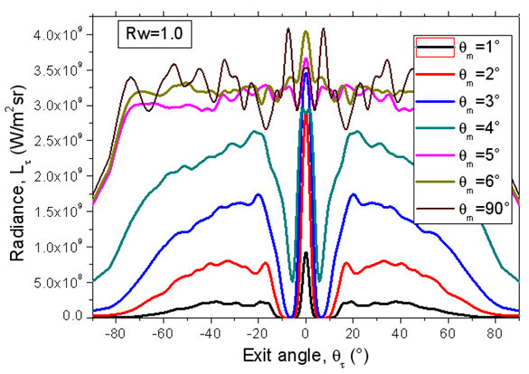 | Figure 19. Cartesian representation of the distribution of the radiance of transmitted flux, when the CPC is irradiated with a lambertian beam with angular divergence  =1°; 2°; 3°; 4°; 5°; 6°; 90°. The wall reflectance is constant and equal to 1.0 =1°; 2°; 3°; 4°; 5°; 6°; 90°. The wall reflectance is constant and equal to 1.0 |
3.7. Average Number of Reflections of Transmitted Rays
- We have previously analyzed the number of reflections made by the transmitted rays as function of
 both as an average on the total flux, and as function on the distance, from the optical axis, of the impact point on the receiver. Now we look at the average number of reflections made by rays transmitted as function of the exit angle
  from the CPC, at different values of the input lambertian divergence
  For this purpose, we have repeated the simulations of radiance shown in Fig. 17 with a different wall reflectance,
  = 0.9. The average number of reflections was obtained by applying the following equation, with
  and
and  = 0.9:
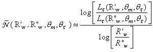 | (20) |
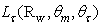 is the radiance of the flux transmitted at angle
  The numbers of output rays do not appear as they were the same at the two wall reflectivities. Fig. 20 shows the polar distribution of
  for angular divergence values
  with 1° steps. There are many interesting features of the polar diagrams of
  to highlight. First of all they are completely developed at
  as it was for the radiance maps (Fig. 17). Then we notice that
  for exit rays close to the optical axis
  these rays do not touch the CPC wall. Then, from
 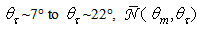 is exactly 1. At higher values of
  grows forming a lobo centered at ~45°, which is narrow at low
  values, with a peak at
  for
for  The lobo then widens occupying the whole range from ~45° to 90°. At
  the rays exit the CPC at
  after one reflection; by increasing
  the reflections increase up to 2.75. One last consideration to do is about the value of
  Whereas the number of reflections of a ray must be exactly an integer, this rarely happens to a mixture of rays, because they have not the same characteristics (same distance x at input aperture and same
  Exceptions are
  at all
  when
when  ~7°÷22° (see Figs. 20a-f), or at
  when
when  (see Figs. 20a,b), or again
  when
when  (see Figs. 20b,c). The diagrams of radiance of Fig. 17 and those of the average number of reflections of Fig. 20 do not clarify, therefore, what are, at the origin, the rays causing a particular radiance or number of reflections profile.
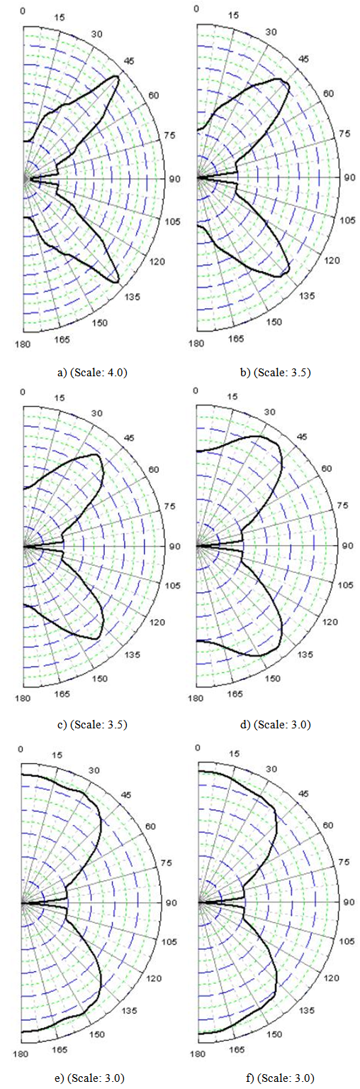 | Figure 20. Polar maps of the average number of reflections of the transmitted rays as function of the exit angle  at different values of the lambertian angular divergence at different values of the lambertian angular divergence  : 1° (a); 2° (b); 3° (c); 4° (d); 5° (e); 6° (f) : 1° (a); 2° (b); 3° (c); 4° (d); 5° (e); 6° (f) |
 interval (0°-5°) in five smaller intervals
  = (0°-1°); (1°-2°); (2°-3°); (3°-4°); (4°-5°), with
  The formula used to calculate the number of reflections is:
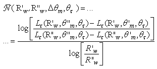 | (21) |
 are those previously simulated with
 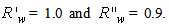 Eq. (21) only requires subtraction of radiance profiles with different
  values. The obtained profiles of
 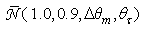 are reported, in Cartesian representation, in Fig. 21, which allows to distinguish better the transmitted rays. Fig. 21 confirms that
  for
for  <7.5° and that
 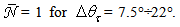 We note also that the various
  profiles consist of bands with the maximum on integer values of
  as desired. The position of these bands
  and their maximum value
  are reported in Tab. 1, as function of
 | Figure 21. Cartesian representation of the average number of reflections of the transmitted rays for an input lambertian beam with angular divergence in the intervals:  =(0°-1°) (black); (1°-2°) (red); (2°-3°) (blue); (3°-4°) (dark cyan); (4°-5°) (magenta) =(0°-1°) (black); (1°-2°) (red); (2°-3°) (blue); (3°-4°) (dark cyan); (4°-5°) (magenta) |
|
 profiles. The bands
  with angular position
  are reported as function of the
  interval
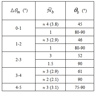
4. Analysis of the Reflected Flux
4.1. Optical Reflection Efficiency
- Let us consider at first the total reflected flux:
 | (22) |
 are the total absorbed and transmitted fluxes, respectively, and
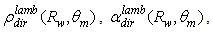
 are the lambertian reflection, absorption and transmission efficiencies, respectively. The total reflected flux can be expressed as function of the radiance
  of the reflected light:
 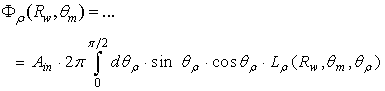 | (23) |
 is the polar angle of the reflected ray. To simulate the reflection properties of the CPC, we have adopted a scheme similar to that used to measure the transmitted light (see Figs. 14, 16), adding a hemispherical screen with
  = 1000 mm radius and ideal absorbance, able to gather all the reflected light from the CPC. The CPC protrudes out of the screen and the center of input aperture meets that of the screen (see Fig. 22).
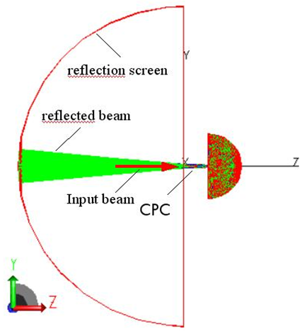 | Figure 22. Scheme of the 3D-CPC irradiated by a lambertian beam with angular divergence  The reflected flux is measured by an absorbing hemispherical screen of radius The reflected flux is measured by an absorbing hemispherical screen of radius  = 1000 mm. The CPC of the figure is not ideal ( = 1000 mm. The CPC of the figure is not ideal ( = 0.9), as consequence, the incident rays (red color) are attenuated after reflection (green color). The output of the CPC has been left open, so the transmitted rays are visible. Most of the transmitted rays are attenuated (green color); the red beam on the z-axis is made of rays crossing undisturbed the CPC = 0.9), as consequence, the incident rays (red color) are attenuated after reflection (green color). The output of the CPC has been left open, so the transmitted rays are visible. Most of the transmitted rays are attenuated (green color); the red beam on the z-axis is made of rays crossing undisturbed the CPC |
 | (24) |
 = 1.0 (black curve), condition for which
  is equal to the ratio between the number of the back-reflected rays to the input rays, because of the absence of optical loss inside the CPC. The reflection efficiency is zero below the acceptance angle, as all the rays are transmitted; then it appears in correspondence of
  (see red curve).
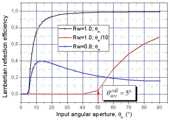 | Figure 23. Lambertian reflection efficiency  of the 3D-CPC calculated for of the 3D-CPC calculated for  and 0.9 wall reflectivity. A portion of the curve of and 0.9 wall reflectivity. A portion of the curve of  is also shown vs. is also shown vs.  (x axis scaled by a factor of 10) (x axis scaled by a factor of 10) |
 for
for  is easily obtained considering that it is simply the complement to 1 of the transmission efficiency
  when
when 
 (see Eq. (7)). We have therefore:
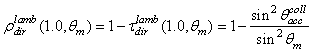 | (25) |
 is quite different from that of
  the reflection efficiency relative to a parallel beam [2]; in that case it was growing rapidly before the acceptance angle, reaching half of its maximum just in correspondence of it. With a lambertian beam,
  is growing more slowly (see Fig. 23) because a part of the beam, that corresponding to
 is always transmitted. From Eq. (25) we see that the limit of
  for
for  is:
is: 
 The reflection efficiency data relative to
  = 0.9 are shown in Fig. 23 (blue curve). While the curve of
  is always growing, the curve of
 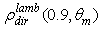 reaches a maximum at
  and then decreases down to 16% for
  being strongly limited by the absorbance of light on the CPC wall.
4.2. Angular Divergence of the Reflected Rays
- The study of the angular divergence of back reflected rays from input aperture has not a practical relevance as it has in the case of the transmitted rays, but it is a useful exercise to apply also to the back reflected rays concepts of the theory of solar concentrators. To simplify the discussion, we limit ourselves to consider an ideal CPC
 As already seen discussing the transmitted flux, the TracePro software produces on the collecting screen a flux map corresponding to the irradiance on the screen wall projected on a plane orthogonal to the z axis. Apart from a dimensional constant factor, equal to
  with
with  radius of the screen and
  input aperture of the CPC, this map is equivalent to that of the radiance of light back reflected by the input aperture, as it has been demonstrated in Eq. (19) for the transmitted flux. The plot of these maps is not necessary, because they are symmetric with respect to the optical axis, and then they give the same information of the profiles of their cross sections.A Cartesian representation of the reflected radiance simulated for some values of
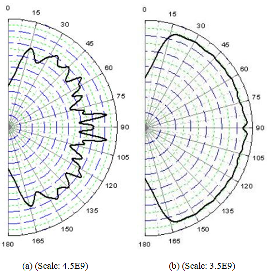
  up to
up to  is shown in Fig. 24. The reflected radiance appears at
  and then grows in intensity reaching a maximum of about 3.2x10⁹ (W/m2sr) at around 12°. Keeping constant in intensity, the radiance band expands then in terms of angular divergence. The envelope of all profiles corresponds to the radiance profile at
  and is characterized by a depression in the center, caused by the “loss” by transmitted rays. This profile, if overturned, form a band of 3.2x10⁹ (W/m2sr) intensity and a width FWHM ≈ 2 x 4.7°. This band definitely has to do with the missing transmitted rays, but it is unexpected that it is equal to ≈ 2 x 4.5° instead of being 2 x
 | Figure 24. Profiles of the reflected radiance vs. the exit reflection angle  simulated for some values of simulated for some values of  from 5° to 20°. The envelope profile gives a reversed band due to the loss by transmitted rays and its FWHM ≈ 2x 4.5°. The wall reflectivity is 1.0 from 5° to 20°. The envelope profile gives a reversed band due to the loss by transmitted rays and its FWHM ≈ 2x 4.5°. The wall reflectivity is 1.0 |
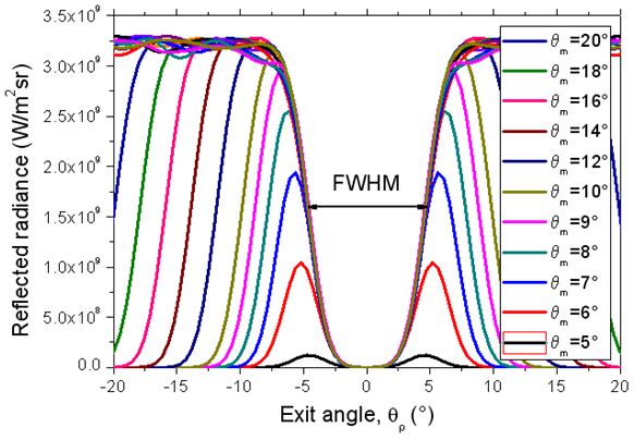
 and their full width at half maximum
  is reported as function of
  The evolution of
  is perfectly linear and is defined by:
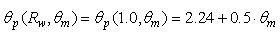 | (26) |
 | Figure 25. Center of the radiance bands  and their full width at half maximum and their full width at half maximum  as function of as function of  |
 is different; after a slow rising up to 10°, the behavior becomes linear and is defined by the function:
 | (27) |
 | (28) |
 therefore, is almost equal to the maximum entrance angle,
  This result is a direct consequence of the Liouville theorem [6], establishing the invariance of the “generalized étendue”, the volume occupied by the system in the phase space, as expressed by Eq. (29) (see also Fig. 26):
 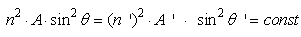 | (29) |
 | Figure 26. Scheme of a generic concentrator with the three main parameters for the input and output apertures: index of refraction, area and angular divergence |
 then we have:
  | (30) |
 | Figure 27. Polar diagrams of the angular distribution of the reflected radiance, simulated for different values of the angular aperture of the lambertian beam at input:  =5° (a); 10° (b); 20° (c); 30° (d); 40° (e); 50° (f); 60° (g); 70° (h); 80° (i); 90° (l). The scale of radiance is expressed in =5° (a); 10° (b); 20° (c); 30° (d); 40° (e); 50° (f); 60° (g); 70° (h); 80° (i); 90° (l). The scale of radiance is expressed in  |
 and an external wall with semi-opening equal to the angular aperture of the lambertian beam
  Cross sections of these beams are then rings with the inner circle growing, at increasing
  from 5° to 12°, and the outer circle from 5° to 90°.
4.3. Average Number of Reflections of the Total Reflected Rays
- To derive the average number of reflections of the total reflected flux,
 it is sufficient to analyze the lambertian reflectance
  at two wall reflectivities and using the formula:
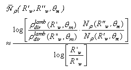 | (31) |
 is the number of reflected rays collected by the screen. The reflection efficiency functions used are those calculated at
  and
and  (see Fig. 23).Fig. 28 shows the curve of
 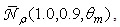 obtained applying Eq. (31) to the pair of reflectivities (1.0; 0.9). The average number of reflections is four at near the acceptance angle (5°) and then grows monotonically reaching up to 16 reflections for
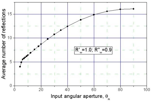 | Figure 28. Average number of internal reflections of the back reflected rays, simulated by applying Eq. (31) for the pair of values of internal wall reflectivity:  |
4.4. Average Number of Reflections Associated to the Reflected Radiance
- As we have done with the transmitted flux, the number of internal reflections of the reflected rays, as function of the exit angle
 at different values of the angular aperture
  can be calculated by simulating the radiance shown in Fig. 27 with a different wall reflectance,
  The average number of reflections
 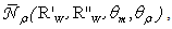 with
with  and
and  was obtained by applying the following equation:
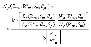 | (32) |
 is the radiance of the flux reflected at
  angle and
  is the number of total reflected rays. The average number of internal reflections of the rays reflected at
  angle is shown in Fig. 29a for
  = 5°, 6°, 8°, 10°, 12°, 18°, 20°, and in Fig. 29b for
  = 30°, 40°, 50°, 60°, 70°, 80°, 90°. It is interesting to note that, apart from the curve corresponding to
  all other curves have a characteristic “V” shape with a minimum of
  equal to ≈5 on the direction of the optical axis of the CPC, and a maximum of
  that grows at increasing
  and falling approximately at
  The results of Fig. 29 are very plausible: the higher the angular divergence of the incoming beam, the greater the number of reflections that the rays experience within the CPC, the greater the exit angle of the rays that make the maximum number of internal reflections. It is also interesting to note that, for exit angles
  all the curves show an increasing trend of
  that is almost linear, particularly for high values of
  (see Fig. 29b). An exception to what has been said so far makes the curve corresponding to
  It shows a constant trend
 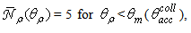 but then decreases with increasing of
  over the value of
  as do all the other curves. With regard to the values of
  they range from about 5 to about 30 and grow at growing
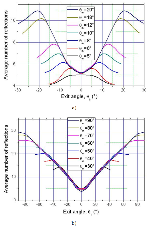
  as illustrated in Fig. 28. Finally, Fig. 30 shows two examples of polar representation of
  for
for 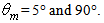
 | Figure 29. Cartesian representation of the average number of internal reflections of the back reflected rays, as function of exit angle  , simulated for , simulated for  Angular aperture of input beam: (a) 5°, 6°, 8°, 10°, 12°, 18°, 20°; (b) 30°, 40°, 50°, 60°, 70°, 80°, 90° Angular aperture of input beam: (a) 5°, 6°, 8°, 10°, 12°, 18°, 20°; (b) 30°, 40°, 50°, 60°, 70°, 80°, 90° |
 | Figure 30. Polar representation of  for for  (a) and 90° (b) (a) and 90° (b) |
5. Analysis of the Absorbed Flux
5.1. Optical Absorption Efficiency
- From the data of transmission efficiency and reflection efficiency we immediately derive the “absorption efficiency” by the expression [1]:
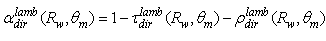 | (33) |
 calculated for the wall reflectivities
  and 0.8, is shown in Fig. 31. The simulation with
  is useless in this case, as it would give a systematic zero absorption efficiency. For
  the absorption of light is due to the internal reflections of mainly the transmitted rays, these reflections being about 2, as we see in Fig. 6.
  | Figure 31. Absorption efficiency  of the 3D-CPC calculated for two wall reflectivities: of the 3D-CPC calculated for two wall reflectivities:  |
 and ≈2x20% when
  as it can be seen in Fig. 31. For
  the absorption of light inside the CPC increases due to the contribution given by the back reflected rays, whose average number of internal reflections increases from 4 to 16 at increasing
 from 4° to 90° (see Fig. 28).
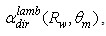
5.2. Distribution of the Absorbed Flux
- Here we study how the absorbed flux is distributed inside the CPC. At this purpose a value of wall reflectivity
 was selected. After each irradiation, by selecting the internal wall of the CPC, the simulation program produces a map of the absorbed flux, projected on the x/y plane orthogonal to the optical axis z. In this way, the map is an annulus with outer radius that of input aperture, a = 12.035 mm, and with inner radius that of output aperture, a’ = 1.052 mm (see Section 2). The intensity map is the projection on the x/y plane of the absorbed irradiation (in W/m2). Some maps of the absorbed flux are shown in Fig. 32 for the wall reflectivity
  a typical value for realistic solar concentrators. The angular aperture of the lambertian beam has been varied from 10° to 90°. From Fig. 32 we can see that the flux density on the wall progressively moves from the exit to the input aperture, and, starting from 60°, the region adjacent to the exit opening is completely devoid of flux.
 | Figure 32. Maps of the flux density on the internal wall, projected on the x/y plane orthogonal to the optical axis z, simulated for different values of the angular aperture of the lambertian beam at input:  = 10° (a); 20° (b); 30° (c); 40° (d); 50° (e); 60° (f); 70° (g); 80° (h) ; 90° (i). Wall reflectivity: = 10° (a); 20° (b); 30° (c); 40° (d); 50° (e); 60° (f); 70° (g); 80° (h) ; 90° (i). Wall reflectivity:  = 0.9 = 0.9 |
 to remove the projection operation made by the program, where α is the angle that the tangent to the CPC profile makes with the optical axis, given by [2]:
 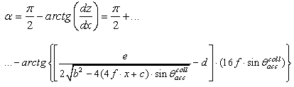 | (34) |
 values, the flux is restricted in a thin zone near the exit opening, with the peak of irradiance increasing and moving towards higher z values at increasing
  For
For  a large band appears in proximity of the input opening and increases at increasing
  remaining centered at about z = 115 mm and leaving a hollow in the center of the CPC. A similar result was observed with parallel beams at input increasing the incidence angle from
  to
to  [2]. For
  values higher than ≈ 30°, this band becomes dominant and most of the flux is absorbed near the input opening (see Fig. 33b). The effect of the increase of the angular divergence of the input beam is ultimately to move much of the flux to the input, as it has been anticipated by the maps of Fig. 32.
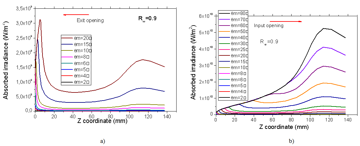 | Figure 33. Distribution of the absorption irradiance along the optical axis, from z = 0 mm (the exit opening) to z = 150 mm (the entrance opening), simulated for angular divergence  from 2° to 20° (a) and from 2° to 80° (b). Wall reflectivity: from 2° to 20° (a) and from 2° to 80° (b). Wall reflectivity:  |
6. Conclusions
- In conclusion, we have presented the results of optical simulations performed on a 3D-CPC nonimaging concentrator, irradiated in direct mode by a lambertian beam. This simulation work is the second discussing the practical applications of the theoretical methods presented in the first part of the series. The “direct” mode of irradiation is here distinguished by the “inverse” mode of irradiation, which will be discussed in a forthcoming part of the series. In this work we analyze the optical properties of the 3D-CPC with canonical shape (no truncation), with an acceptance angle at collimated light of 5° and maximum exit angle of 90°. The CPC has been analyzed in extreme detail by using a ray-tracing program. We have explored its transmission properties, those of the most practical importance when the 3D-CPC is used in a solar system, in terms of transmission efficiency, spatial and angular distribution of the flux at the output. Generally of less importance is the study of its reflection and absorption properties. Nevertheless, we have dedicated a large part of this paper also to these aspects, applying the same methods used for the transmitted light, because it helps to understand the secret mechanism of light concentration in a CPC. In the previous work of this series, we have analyzed the optical properties of the CPC irradiated by a collimated beam, oriented at different polar angles respect to the optical axis. In the actual work, we have just modified the geometry of the input beam, using a lambertian beam, that is a beam with cylindrical symmetry and constant radiance. This allowed us to obtain cylindrically symmetric beams at output of the CPC, that have facilitated the elaboration of the results, and to introduce new optical quantities, some already defined in the first theoretical work, others defined for the first time in this work. As in this work we have dealt with the CPC as if it were a generic optical element, we believe it will help to introduce into the routine work of the optical design new methods of simulation to be applied universally to the optical devices.