Madhusmita Mishra1, Sarat Kumar Patra1, Ashok Kumar Turuk2
1EC Department, National Institute of Technology, Rourkela, Odisha, India
2CS Department, National Institute of Technology, Rourkela, Odisha, India
Correspondence to: Madhusmita Mishra, EC Department, National Institute of Technology, Rourkela, Odisha, India.
| Email: |  |
Copyright © 2015 Scientific & Academic Publishing. All Rights Reserved.
Abstract
This work is concentrating on generating gamma-gamma turbulence model taking into consideration the Forward method, Matsuno method, Huen method, Runge-Kutta 2 method (mid-point), Runge-Kutta 4 method, Adams-Bashforth 2 method (extrapolates P, Z in time), Adams-Bashforth 3 method (extrapolates P, Z in time), Quasi-Adams-Bashforth 2 method (extrapolates P, Z in time) and Adams-Moulton 3 method. Where P stands for atmospheric pressure and Z stands for atmospheric height. Analyzing the gamma-gamma pdf for smaller and larger separation of time-scale regimes using stability and skewness criterion, we concluded that the Matsuno and Quasi-Adams-Bashforth 2 methods are suitable for generating accurate gamma-gamma turbulence model.
Keywords:
Forward, Matsuno, Huen, Runge-Kutta 2 (RK2), Runge-Kutta4 (RK4), Adams-Bashforth 2 (AB2), Adams Bashforth 3 (AB3), Quasi-Adams-Bashforth 2 (QAB2), Adams-Moulton 3 (AM3)
Cite this paper: Madhusmita Mishra, Sarat Kumar Patra, Ashok Kumar Turuk, Modified Gamma-Gamma Turbulence Model Using Numerical Integration Methods, International Journal of Optics and Applications, Vol. 5 No. 3, 2015, pp. 71-81. doi: 10.5923/j.optics.20150503.04.
1. Introduction
The lower layer of air surrounding the earth's surface gets warmed up due to solar radiation absorption and thus become less dense than the air at higher altitude. The rising movement of less dense air and the surrounding cooler air mix turbulently to cause random fluctuation in air temperature. This causes inhomogeneities in the form of discrete cells or eddies and refractive prisms of different sizes and indices of refraction. When information bearing optical beam passes through this kind of turbulent medium, its phase and amplitude varies randomly. This phenomenon is called scintillation. Scintillation results in faded received optical power and thus leads to system performance degradation. Different indices of refraction create optical turbulence. Optical turbulence leads to irradiance fluctuations, beam broadening and loss of spatial coherence of the optical wave. This work concentrates on intensity modulated direct detection based OWC system and for this system the irradiance fluctuation matters a lot. Hence for modeling purpose this work is concentrating only on turbulence induced fluctuation of the received optical power (irradiance). Usually atmospheric turbulence is categorized in the regimes that are function of travelled distance through the atmosphere by the information bearing optical wave. Depending on the magnitude of inhomogeneities and index of refraction variation the regimes are classified as weak, moderate, strong and saturation. To model this turbulent medium as a channel, its characteristics must be well understood. The characteristics of a channel are well understood by means of its impulse response. For modeling the turbulent medium it is imperative to describe the pdf statistics of the irradiance fluctuation. The models log-normal, gamma-gamma and negative exponential are used respectively for weak, weak to strong and saturate regimes. However, this work is limited to gamma-gamma turbulence model [1, 2]. To the best of our knowledge, this is the first work that is applying numerical integration methods to modify the gamma-gamma turbulence model. Here we have used the numerical integration techniques like; Forward method, Matsuno method, Huen method, Runge-Kutta 2 (mid-point method), Runge-Kutta4, Adams-Bashforth 2 (extrapolates P, Z in time), Adams-Bashforth 3 (extrapolates P, Z in time), Quasi-Adams-Bashforth 2 (extrapolates P, Z in time) and Adams-Moulton 3 method. Where P stands for atmospheric pressure and Z stands for atmospheric height [3-9]. Analyzing the gamma-gamma pdf for weak and strong turbulence regimes using stability and skewness criterion, we have concluded that the Matsuno method and Quasi-Adams-Bashforth 2 methods are suitable for generating accurate gamma-gamma turbulence model.The rest of the paper is organized as follows. Section II describes modeling of the turbulent scenario. Section III gives an insight into the investigation of the gamma-gamma turbulence model using various numerical integration methods. Section IV gives the result analysis and discussion. Section V provides the concluding remarks.
2. Modelling of the Turbulent Scenario
The turbulent scenario can be modeled according to the following steps [10, 11]:• Refractive index fluctuation in terms of atmospheric temperature variation: The optical turbulence due to refractive index fluctuation is equivalent to direct end product of random variations in atmospheric temperature from one point to other.• Modeling the atmospheric temperature variation: The random temperature change in atmosphere is a function of the altitude, atmospheric pressure and wind speed. During the modeling process the smallest turbulent eddies are termed as inner scale  and the largest turbulent eddies are termed as outer scale
  The atmospheric temperature and its refractive index are related as:
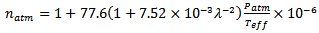 | (1) |
Where  is the atmospheric refractive index,
  is the pressure of atmosphere in millibars,
  denotes the effective temperature in Kelvin and
  denotes the wavelength in microns.• Modeling the amount of refractive index fluctuation:According to Kolmogorov, amount of refractive index fluctuation is characterized by the index of refraction structure parameter
  is a function of the atmospheric altitude, wavelength and temperature.This work is concentrating on gamma-gamma turbulence model taking into consideration the Forward method, Matsuno method (forward/backward), Huen method (forward/trapezoidal), Runge-Kutta 2 (mid-point method), Runge-Kutta 4 method, Adams-Bashforth 2 method (extrapolates P, Z in time), Adams-Bashforth 3 method (extrapolates P, Z in time), Quasi-Adams-Bashforth 2 method (extrapolates P, Z in time) and Adams-Moulton 3 method. Where P stands for atmospheric pressure and Z stands for atmospheric height. The next section gives an insight into the investigation of the gamma-gamma turbulence model using various numerical integration methods using stability and skewness criterion.
3. Investigation of the Gamma-Gamma Turbulence Model Using Various Numerical Integration Methods
In [1, 2], the unconditional gamma-gamma distribution function is obtained as: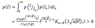 | (2) |
Where  and
and  represents the effective number of large and small scale eddies,
  represents modified bessel’s function of the second kind of order
  and
and  represents the gamma function.
  denotes the irradiance of eddies due to large scale turbulence.
  denotes the normalized received irradiance.The key idea of this work lies in the following fact. Since the
  and
and  are related to the index of refraction structure parameter with respect to height and pressure. Hence we can modify the
  in the equation (2) by taking solutions of the equations (3) and (4) given below using any one of the numerical integration methods such as: Forward method, Matsuno method (forward/backward), Huen method (forward/trapezoidal), Runge-Kutta 2 (mid-point method), Runge-Kutta 4, Adams-Bashforth 2 (extrapolates
  in time), Adams-Bashforth 3 (extrapolates
  in time), Quasi-Adams-Bashforth 2 (extrapolates
  in time) and Adams- Moulton method. Where
  stands for atmospheric pressure and
  stands for atmospheric height.
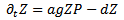 | (3) |
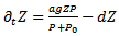 | (4) |
In equations (3) and (4),  and
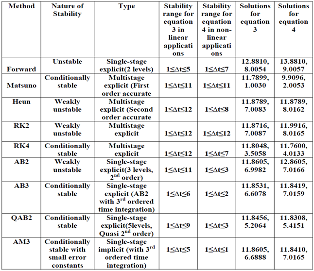
and  are constants. The equation (3) corresponds to a linear model and the equation (4) corresponds to a non-linear model that means there is wider separation of inherent time scales.Using the various numerical integration methods, the gamma-gamma turbulence scenarios for the largest value of the time scales are shown in Fig.1-18. Fig.1-9 and Fig.10-18 are obtained following the solutions of equation 3 and 4 respectively. TABLE–1 shows the types, stability criterions of these numerical integration methods and the solutions of the equations 3 and 4, when they are applied. The Fig. 19 shows the gamma-gamma pdf using the various numerical integration methods for evaluating the solutions of equation 3. The Fig. 20 shows the gamma-gamma pdf using the various numerical integration methods for evaluating the solutions of equation 4.
Table 1. Characteristics, stability and solutions of the numerical integration methods, when applied to the turbulent scenario
 |
| |
|
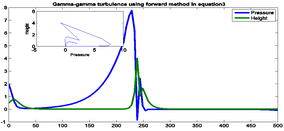 | Figure 1. Gamma-gamma turbulence using Forward method in equation 3 |
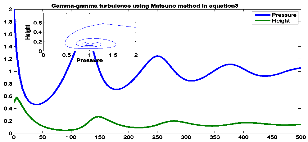 | Figure 2. Gamma-gamma turbulence using Matsuno method in equation 3 |
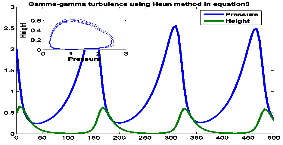 | Figure 3. Gamma-gamma turbulence using Heun method in equation 3 |
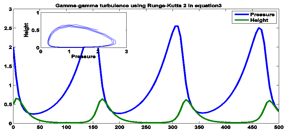 | Figure 4. Gamma-gamma turbulence using Runge-Kutta 2 method in equation 3 |
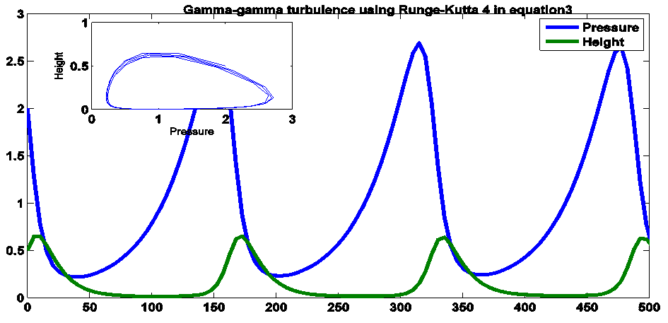 | Figure 5. Gamma-gamma turbulence using Runge-Kutta 4 method in equation 3 |
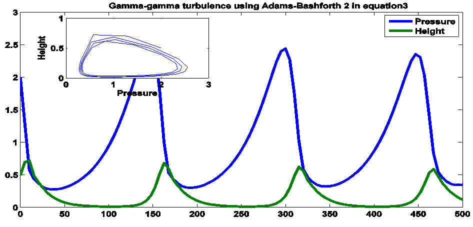 | Figure 6. Gamma-gamma turbulence using Adams-Bashforth 2 method in equation 3 |
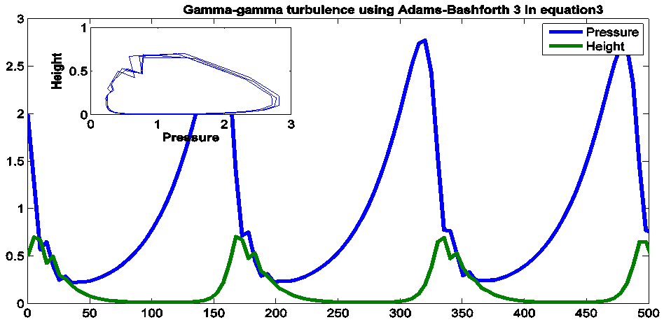 | Figure 7. Gamma-gamma turbulence using Adams-Bashforth 3 method in equation 3 |
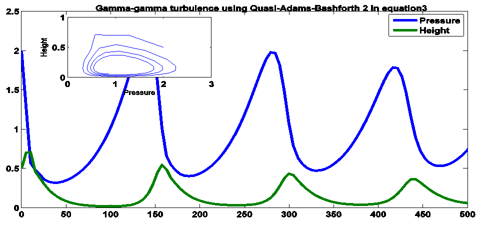 | Figure 8. Gamma-gamma turbulence using Quasi-Adams-Bashforth 2 method in equation 3 |
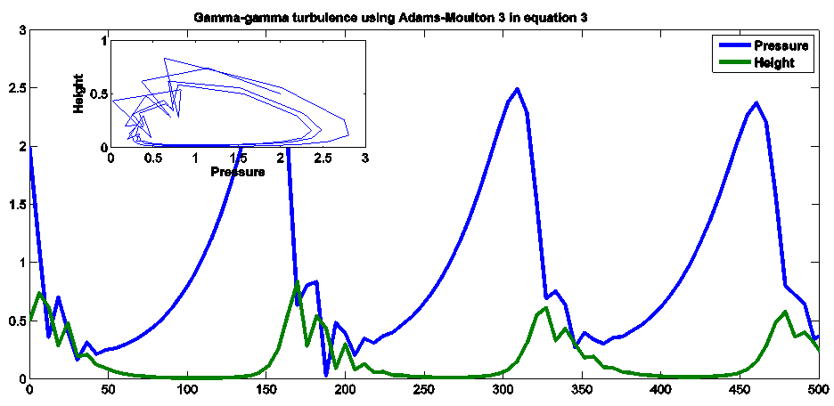 | Figure 9. Gamma-gamma turbulence using Adams-Moulton 3 method in equation 3 |
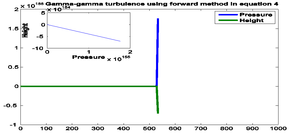 | Figure 10. Gamma-gamma turbulence using forward method in equation 4 |
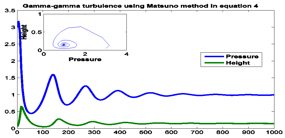 | Figure 11. Gamma-gamma turbulence using Matsuno method in equation 4 |
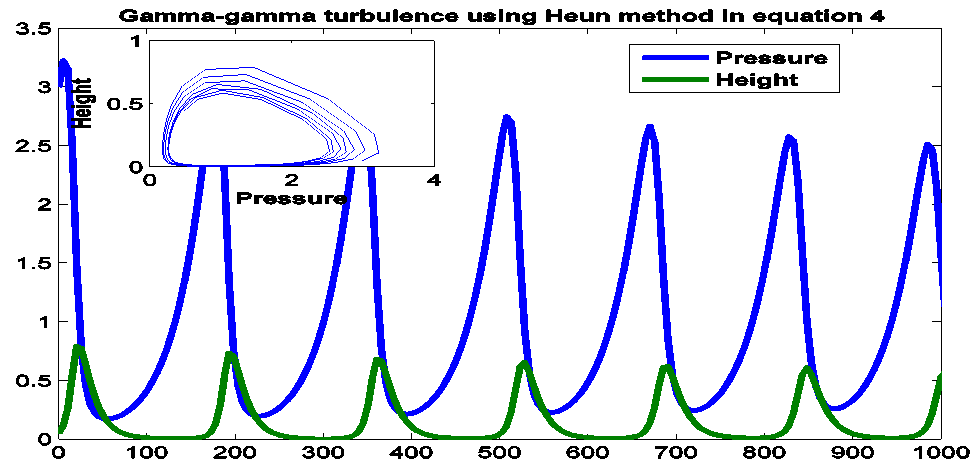 | Figure 12. Gamma-gamma turbulence using Heun method in equation 4 |
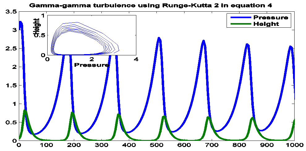 | Figure 13. Gamma-gamma turbulence using Runge-Kutta 2 method in equation 4 |
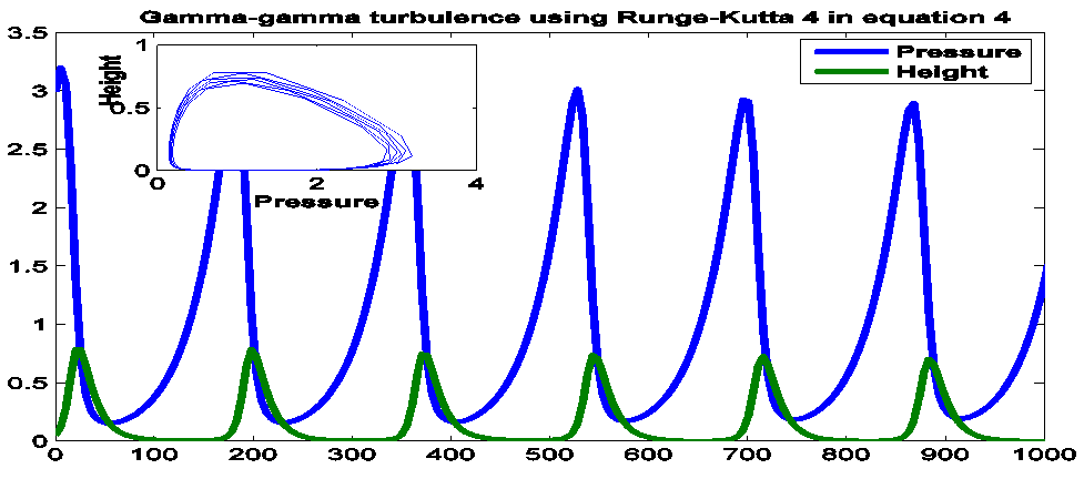 | Figure 14. Gamma-gamma turbulence using Runge-Kutta 4 method in equation 4 |
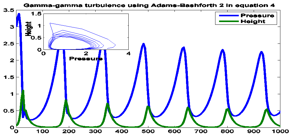 | Figure 15. Gamma-gamma turbulence using Adams-Bashforth 2 method in equation 4 |
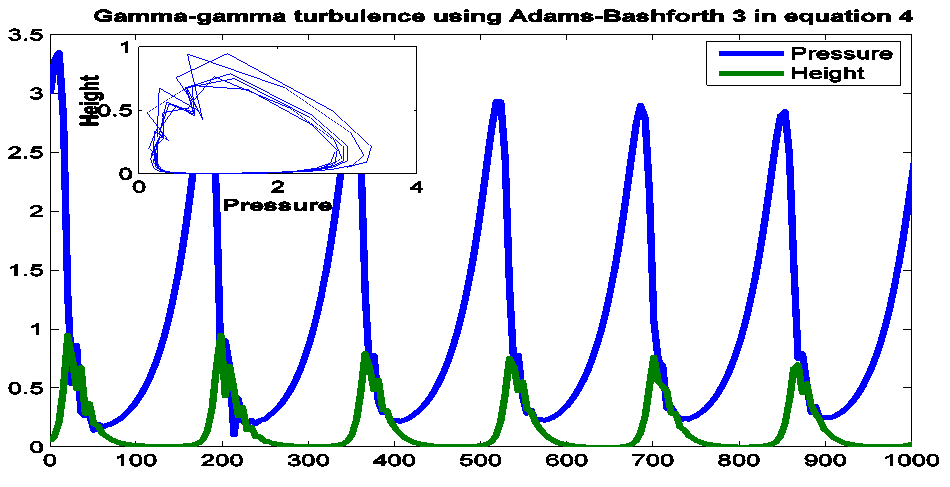 | Figure 16. Gamma-gamma turbulence using Adams-Bashforth 3 method in equation 4 |
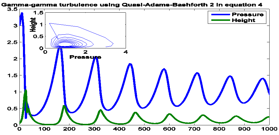 | Figure 17. Gamma-gamma turbulence using Quasi-Adams-Bashforth 2 method in equation 4 |
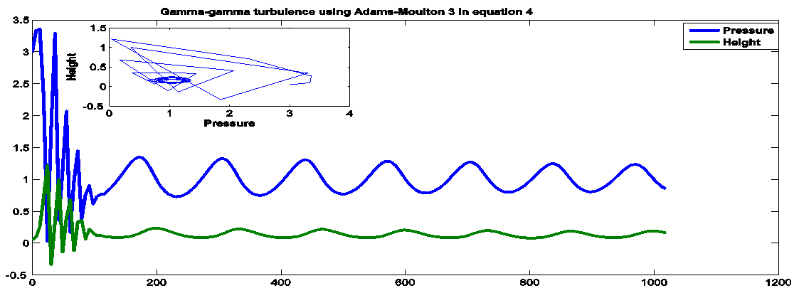 | Figure 18. Gamma-gamma turbulence using Adams-Moulton 3 method in equation 4 |
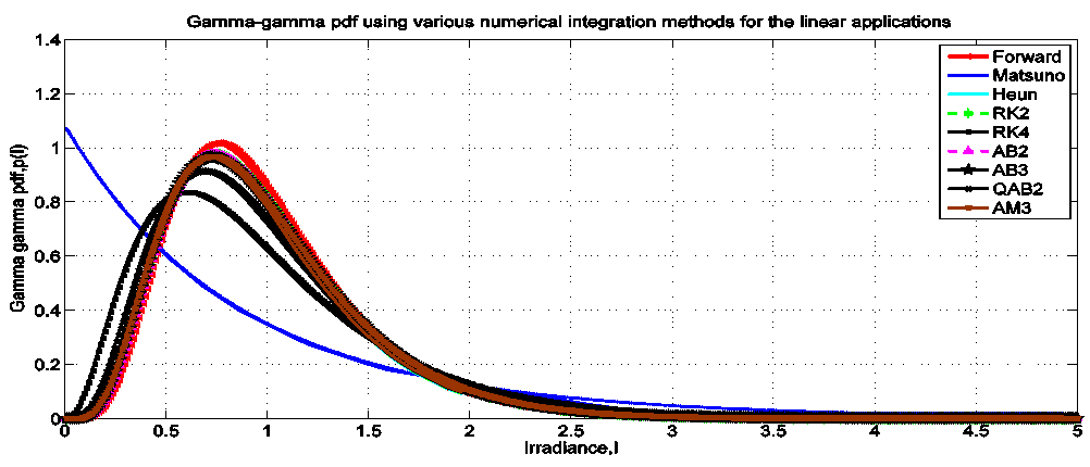 | Figure 19. Gamma- gamma pdf using various numerical integration methods for the linear applications |
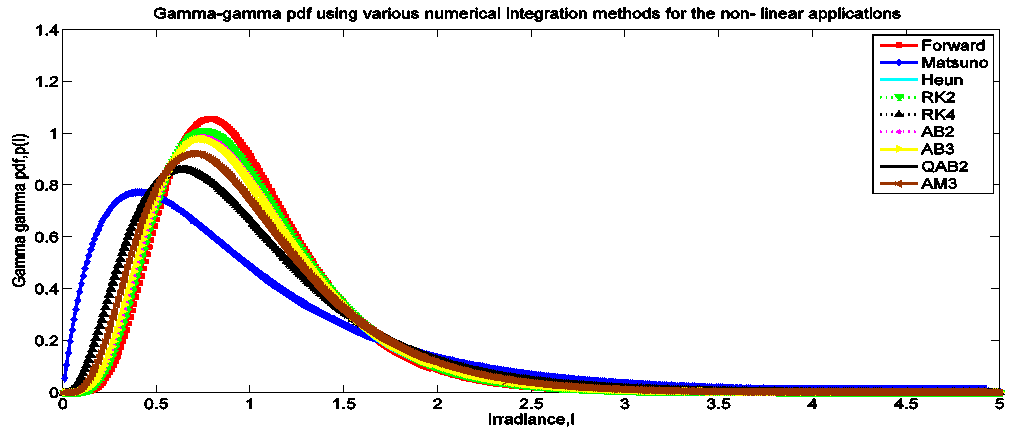 | Figure 20. Gamma- gamma pdf using various numerical integration methods for the non-linear applications |
4. Result Analysis and Discussion
A. Analysis in comparison to previous methods of modelingPreviously  and
and  were calculated taking into consideration the horizontal distance travelled by the optical beam in the medium. But, here we have taken into consideration the pressure and height through which thebeam has covered the medium. Consideration of pressure and height will give more dimensional view of the turbulent scenario. This turbulent scenarios are shown in Fig. 1-9 and Fig. 10-18 using various numerical integration methods for linear and non-linear applications respectively. By using the numerical integration methods, the gamma-gamma distribution will be bounded as there is increase in turbulence. This is because of the consideration of the solutions by taking the largest stable value in the time scale. The largest stable values for various numerical integration methods are shown in TABLE-1. In contrast to this, in the previous method of modeling, the gamma-gamma distribution was approaching negative exponential distribution as there is increase in turbulence [1, 2].B. Current result analysis and discussionHere we have considered linear and non-linear applications of the turbulent channel. In both of the cases, among all the multistage explicit and single stage explicit schemes, the Matsuno method is found to be more suitable for gamma-gamma turbulence modelling. This is because of the fact that using the Matsuno method the perturbations are not growing in time. This is clearly visible in Fig.2 and Fig.11 for linear and non-linear cases respectively. As far as stability criterion is considered, this method is conditionally stable and gives equal range of stability for both linear and non-linear applications. This is shown in TABLE-1. Since it is first order accurate, any channel equation represented as partial differential equation (PDE) can be successfully solved. Since it is a multistage explicit method, there is no risk of the computational mode which arises in single stage explicit schemes with higher number of time levels. Compared with all other single stage explicit methods as listed in TABLE-1, the Quasi-Adams-Bashforth 2 method can be suitable for gamma-gamma turbulence modelling. This is because of the following facts. Firstly, compared to all other single stage explicit schemes, the perturbations are not growing in time. Secondly, as there is increase in the irradiance, the gamma-gamma distribution plot is more skewed. This scenario is clearly visible in Fig.19 and Fig.20 for linear and non-linear applications respectively. From Fig. 7-9, Fig.16-18 and TABLE-1, it is clear that, Adams-Moulton 3 method is showing smaller error constants as compared to Adams-Bashforth 3 method and stability range nearly equivalent to Quasi-Adams-Bashforth 2 method. But, in Fig.9 and Fig.18, the perturbations of Adams-Moulton 3 method are not decreasing in time. Hence, Adams-Moulton 3 method can not be considered as a good candidate for for gamma-gamma turbulence modelling. C. Future research directionsEvery work has its own advantage and disadvantages. Hence within certain limitations, this work has the following research directions:• The Adams-Bashforth method in first step and Adams-Moulton method in the second step can be used as a predictor- corrector formulae to increase the accuracy and stability range in more non-linear modelling applications.• The accurate gamma-gamma model generated in this work can be used in the performance analysis of various signal processing techniques and channel coding techniques over free- space optical communication link.
5. Conclusions
The gamma-gamma turbulence model has been studied and analyzed through the numerical integration methods. The various numerical integration methods have been compared basing on the stability, type and linear or non-linear applications. We found the Matsuno method to be suitable for generating accurate gamma-gamma turbulence model for both linear and non-linear applications. Nextly, the QAB2 scheme among the single- stage explicit schemes is found suitable for gamma-gamma turbulence modeling. The consideration of numerical integration methods along with stability criterion and skewness has made the gamma-gamma distribution bounded when there is an increase in turbulence.
References
| [1] | W.O.Popoola," Subcarrier intensity modulated free-space optical communication systems", PhD thesis, University of Northumbria, September 2009. |
| [2] | E.T. Fabiyi, X. Tang, Z. Ghassemlooy, M. Mansour Abadi, W.O. Popoola" Performances of Free Space Optical Link under a Controlled Atmospheric Turbulence Channel", Symposium on the Convergence of Telecommunications, Network and Broadcasting, 23-24 June 2014. |
| [3] | Kristofer Döös and Laurent Brodeau," Numerical Methods in Meteorology and Oceanography", Stockholm University , March 10, 2014. |
| [4] | Lecture 5, “12.950 Atmospheric and Oceanic Modeling”, MIT, Spring, 2004. |
| [5] | Richard B. Rood, "Numerical advection algorithms and their role in atmospehric transport and chemistry models ", Reviews of Geophysics, Vol.25, February, 1987. |
| [6] | J.C. Chiou, S.D. Wu, “On the generation of higher order numerical integration methods using lower order Adams-Bashforth and Adams-Moulton methods”, Journal of Computational and Applied Mathematics Elsevier, pp. 19-29, 108 (1999). |
| [7] | Peter Arbenz, “Numerical Methods for Computational Science and Engineering”, Lecture 26, Dec 16, 2013. |
| [8] | Pavla Sehnalová, “Stability and Convergence of Numerical Computations”, Information Sciences and Technologies Bulletin of the ACM Slovakia, pp. 26-35, Vol. 3, No. 3 (2011). |
| [9] | Nikesh S. Dattani, “Linear Multistep Numerical Methods for Ordinary Differential Equations”, October 28, 2008. |
| [10] | Larry C. Andrews, Ronald L. Phillips, "Laser Beam Propagation through Random Media, Second Edition", 16 September 2005. |
| [11] | Mohammad Ali Khalighi, Murat Uysal, " Survey on Free Space Optical Communication: A Communication Theory Perspective ", IEEE Communication Surveys & Tutorials, vol. 16, no. 4, Fourth Quarter, 2014. |
 Abstract
 Reference
 Full-Text PDF
 Full-text HTML