1. Introduction

Due to its high Finesse characteristic, Optic Ring Resonator (ORR) has become a main focus in optical device researches such as in wavelength selective switches [1], add-drop filters [2], biosensors [3], dynamic characteristics [4], single-frequency lasers [5], single and multi structures [6-11], multi inputs [12]. Many ORR researches utilized fiber to form the ring as Fiber ORR (FORR) and published their results on coherence effect [13], dynamic resonance characteristic [14], ringing phenomenon [15], bistability and instability [16], fiber bragg grating filter [17], simultaneous resonance with double couplers [18], optical vernier filter [19], transmission characteristics and sensitivity [20-21], erbium doped fiber ring laser [22] and for gyroscope aplication as well [23], temperature sensors and transducers [24], gas detection such as hydrogen sensor [25-27] and other optochemical sensors [29]. All of these show that FORR is still interesting research theme in the optical technology research, in addition to its simplicity to utilize it.

In 1982, Stokes et al [16] presented their analytic research of FORR in which one fiber optic is formed a ring with parts closed each other as shown in Figure 1.a hereinafter referred to as Cross type FORR (CFORR). In his paper Stokes mentioned that the characteristics of output is change as the intensity loss, varies, where the Finesse decreases as the intensity loss increases (=0.05, 0.10) [16]. However, Stokes did not make any characteristic change based on variation.

In 2012, Seraji et al. [29] used their own formulations and performed a comparison between cross- and direct coupled FORR as shown in Figure 1.b. He concluded that the Finesse of CFORR increases as increases (by varying = 0.35, 0.55, 0.75, 0.95), while for Direct type FORR (DFORR), the Finesse decreases as the increases (by varying = 0.05, 0.25, 0.45, 0.65). For more, he concluded that the loop intensity of cross type is nearly double of its direct type.

In this paper, we conduct an analysis of the two configurations based on Stokes’ formula [16] and showing the characteristic intensities for both configurations, especially for the peaks and dips at resonance condition when varies (= 0.01 until 0.99 with interval of 0.01). It is shown that their relations to is not linear, and they exhibit an opposite phenomena to each other. We explore further with an experiment utilizing Polarization Maintained Fiber (PMF) and show that DFORR shows better Finesse than that of CFORR, and will be published in a separate paper.

2. CFORR and Its Response Formula

To understand the working principles of FORR, we conduct simulation and experiment utilizing a 2x2 coupler (2 inputs and 2 outputs) to form a ring resonator as shown in Figure 1. Signal, , passes into a single coupler with coupling ratio, , the signal is split into 2 directional output within the coupler, a part of the signal is directed to the output port as and the other part is directed into the loop and will be sent back to get through the coupler again. The form of waveguides inside the coupler are different where as Figure 1. a shows a cross type coupler and Figure 1b show a direct type one. This difference of structure, then, reflects the response formula as will be discussed below.

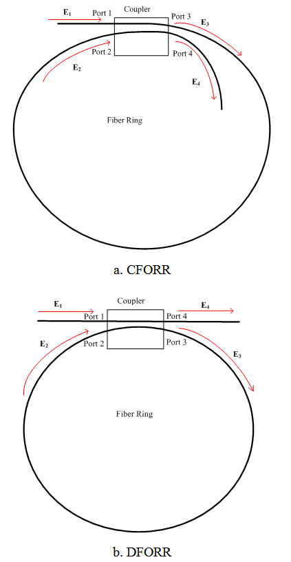Figure 1. Schematic diagram of FORR with single coupler

2.1. Intensities of Output and Loop for CFORR

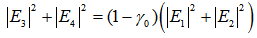
Cross type configuration is the beginning of the research associated with FORR, since it is easy to form a ring with only 1 single fiber and bring certain parts of each end of the fiber close to each other, as illustrated in Figure 1.a, thus the evanescent mode of the circulating light gets coupled to the nearby fiber optic.

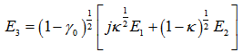
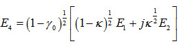
Directional coupler is modeled as an ideal device with no loss, but with an additional fractional intensity loss, , that independent to coupling coefficient, . Thus, under steady state operation, the relation of complex amplitude of electric fields of light at each port (port 1 ~ port 4) may be expressed as [16]:

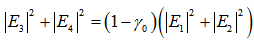(2.1)

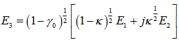(2.2)

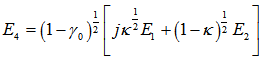(2.3)

where, is the amplitude of complex field at i-th port, is the power coupling coefficient of the coupler. = 0 when totally there is no coupling, and =1 means perfect cross coupling occurs. and are then related through:

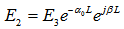
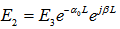(2.4)

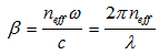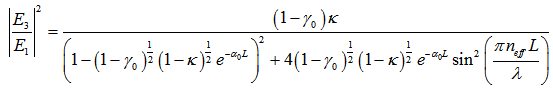
with , is the amplitude attenuation coefficient of the fiber, is the effective refractive index of the fiber, is the optical frequency, is the speed of the light and is the fiber ring’s length. By utilizing equations (2.2), (2.3), (2.4), we may derive at port 3 and at port 4 that contains , , , and as: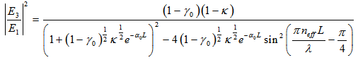

(2.5)

(2.6)

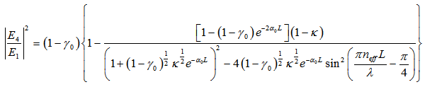
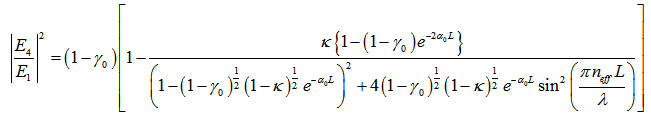
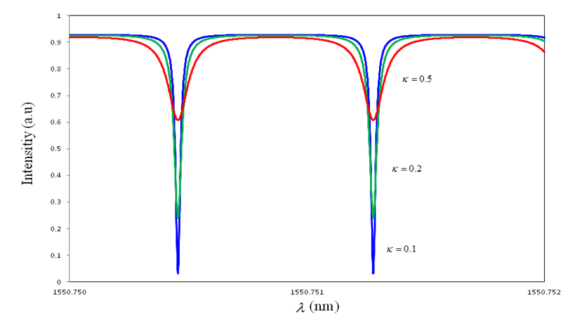
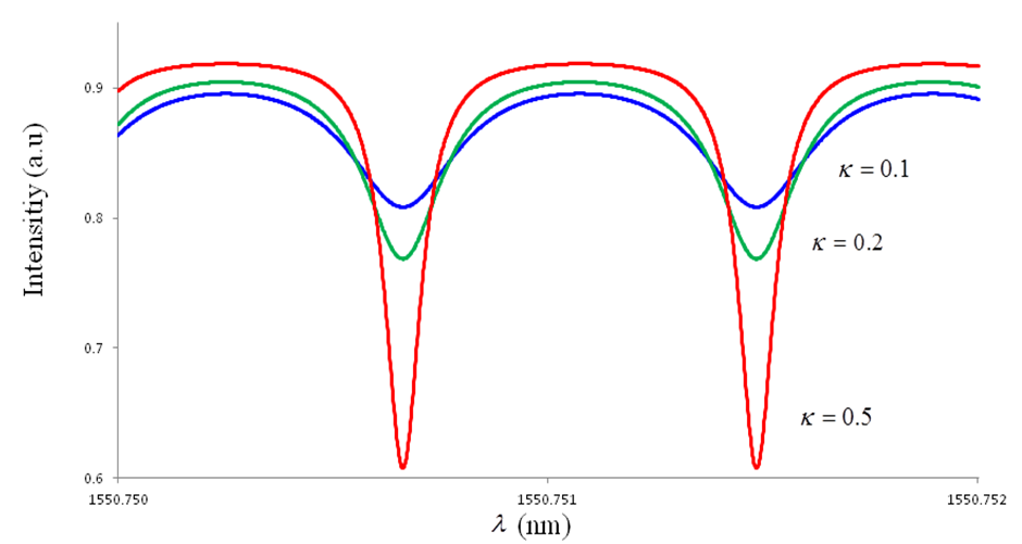
in Eq. (2.5) is known also as the normalized loop intensity, , of light entering into the ring resonator, while as in Eq. (2.6) is known as the normalized output intensity of the system. Then, and may be shown as in Figure 2 and 3 respectively, where we set (typical value: 5% ~ 10%), = 0.1, 0.2 and 0.5.

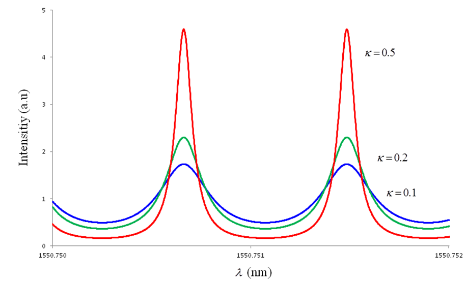Figure 2. Graph for CFORR

Figure 3. Graph for CFORR

2.2. Resonance Condition for CFORR

The resonance condition of the configuration may be achieved when becomes maximum and at the same time, is 0. The former may be reached if and only if 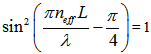, thus:

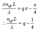(2.7)

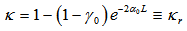
where is integer. Furthermore, the resonance may be happens when the resonant coupling coefficient, , fulfils a requirement as:

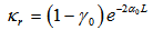(2.8)

Considering the Eq. (2.8), at resonance, the of Eq. (2.5) becomes:

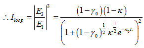(2.9)

or

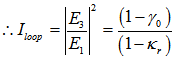(2.10)

3. DFORR and Its Response Formula

Seraji et al [29], specifically addressed it in 2012, and conducted its comparison with the CFORR for some values. Based on Stokes formulation for the CFORR, we conduct analytical work for DFORR and present the amplitude fields of light interaction at port 1~4. It is described in relations mentioned bellow:

3.1. Intensities of Output and Loop of DFORR

With almost similar situation as mentioned in the previous section, we describe the complex amplitude of mode interaction as follows:

(3.1)

(3.2)

(3.3)

Meanwhile the complex amplitude at Port 2 may only be related to that one of Port 4, where the light there may only experiences attenuation loss due to fiber characteristic and fractional loss. Thus, it can be expressed as:

(3.4)

by manipulating the above equations with the same procedure as mentioned in the previous section, we obtain the normalized loop and output intensities as follows:

(3.5)

(3.6)

3.2. Resonance Condition for DFORR

The resonance condition of the configuration may be achieved when becomes maximum and at the same time, is 0. The former may be reached if and only if 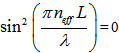, thus at this condition we may gain:

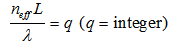(3.7)

(3.8)

is defined as the coupling coefficient at resonance condition. Furthermore, the normalized loop and output intensities may be derived respectively as:

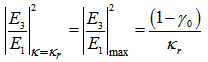(3.9)

The results of the normalized and intensities are shown in Figure 4 and 5 respectively, with= 0.07 and = 0.1, 0.2, 0.5.

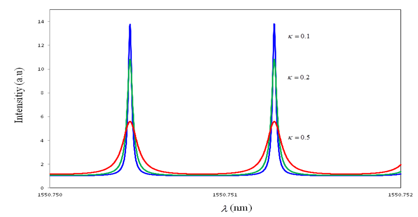Figure 4. Graph for DFORR

Figure 5. Graph for DFORR

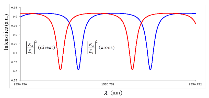
4.Comparison of Output and Loop Intensities for Both Configurations

We present the comparison for both type configurations in this section. We vary the value from 0.01 until 0.99 with interval of 0.01, then we compare the intensities, and for both configurations. With varies 0.01 ~ 0.99, and reaches their first resonant points at=1,550.75066 nm and 1,550.75046 nm for CFORR and DFORR respectively, i.e., the peak or dip of DFORR slightly precedes than that of CFORR by = 2.06x10^-4 nm, and for more, they exhibit different behaviours.

Figure 6 and 7 shows the comparison of and respectively, for = 0.5. With = 0.5, then the for DFORR has Free Spectral Range (FSR) = 8.22x10^-4 nm which is exactly the same as that one of CFORR, and Full Width at Half Maximum (FWHM) = 1.27x10^-4 nm which is 0.25x10^-4 nm wider than that of CFORR. Meanwhile has FSR = 8.22x10^-4 nm, which is the same value with that of CFORR but FWHM = 4.68x10^-4 nm, which is slightly 0.01x10^-4 nm narrower than that of the CFORR. This means that at = 0.5, the Finesse of DFORR is slightly bigger by 4x10^-3 more than that of CFORR.

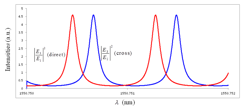Figure 6. Graph for CFORR and DFORR, when κ = 0.5

Figure 7. Graph for CFORR and DFORR, when κ = 0.5

The maximum point for (peak, dashed line) and the minimum point for (dip, solid line) when CFORR (blue) and DFORR (brown) at resonance are shown at Figure 8, as the varies 0.01 ~ 0.99.

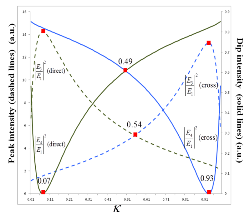Figure 8. Graph (dashed line) and (solid line) at resonant conditions for CFORR (blue) and DFORR (brown)

As shown in the graphic, peak intensity of CFORR, (dashed blue line), increases gradually with the increasing of value, and after passing through at point of about = 0.67, it rises more steeply until it reaches its maximum at point of = 0.93, and then drops drastically for the rest high value. In contrast to this, dip intensity of CFORR (solid blue line) decreases slowly with the increasing of value, and after passing through at point of about = 0.67, it decreases more sharply until it reaches its minimum at point of = 0.93, henceforth rises steeply for the rest of high value.

The significance of this graph is, when CFORR is utilized as sensor device by treating changes to its value through the application of external perturbation etc., then the best operating area is for at around 0.67 ~ 0.99.

Meanwhile, for DFORR, on contrary, the peak intensity, (dashed brown line), increases sharply with the increasing of , and after reaching its maximum at point of = 0.07, it falls relatively sharp until = 0.33, for thereafter decreases more gradually for the rest high value. Furthermore, on the other hand, the dip intensity, (solid brown line) decreases drastically with the increasing of value, and after reaching its minimum at point of = 0.07, it increases more steeply until passing through point of = 0.33, and henceforth rises more gradually for the rest of high value.

The significance of this graph is when it is utilized as sensor device by treating changes to its value, so the best operating boundaries for its value is at around 0.01 ~ 0.33.

Furthermore, the for both CFORR and DFORR have the same value when reaches around 0.55, meanwhile for both configurations have the same value when reaches 0.49. This concludes that when the value of is around 0.5, analytically both configurations exhibit the same phenomena. In addition, during steady state condition, when there is no external perturbation that may be applied to change the of the system, CFORR shows much better performance compared to DFORR, by the use of value at around 0.01 ~ 0.49. Meanwhile, DFORR shows much better performance with the use of value around 0.49 ~ 0.99.

We have conducted some experimental works as well, where Polarization Maintained Fiber, with 2x2 coupler of 50/50 is utilized to construct ring resonator of 2 m in length. We used Tunable Laser Source (TLS) as the light source and Optical Spectrum Analyzer (OSA) for the detection of the output intensity. The result for CFORR and DFORR is shown in Figure 9, where DFORR exhibits much better Finesse than that of CFORR. There are several dips appears with FSR around 1.7 ~ 3.6x10^-4 nm. This inconsistency dips may occurs due to multiple misalignment wavelength interaction between light going direct to output port and light comes out after traveling inside the ring which is not always in the same phase to each other. Further discussion regarding to this experimental result will be published separately.

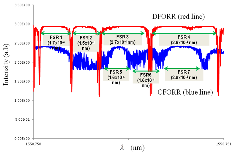Figure 9. Experimental Work Utilizing PMF with 50:50 Coupler

5. Conclusions

We have conducted a more detailed analytical work of (normalized loop intensity) and (normalized output intensity) performance, compared to previous work, where the coupling coefficient of utilized coupler, , is varied 0.01~0.99.

The significance of this graph is, when CFORR is utilized as sensor device by treating changes to its value through the application of external perturbation etc., then the best operating area is for at around 0.67 ~ 0.99. On contrary, when DFORR is utilized as sensor device by treating changes to its value, so the best operating boundaries for its value is at around 0.01 ~ 0.33. During steady state condition, when there is no external perturbation that may be applied to change the of the system, CFORR shows much better performance compared to DFORR, by the use of value at around 0.01~0.49. Meanwhile, DFORR shows much better performance with the use of value around 0.49~0.99. Experimental work has been conducted to confirm the phenomena. We gain some FSR with the same orde with analytical work, but further discussion will be published in a separate paper.

The results mentioned above also confirm that both configurations perform opposite situation to each other, and we may consider this situation for utilizing the best configuration for both. The analytical result gained in this work can be useful for the selection of configuration and purpose of FORR utilization.