Said Amar, Mustapha Bahich, ElMostapha Barj, Mohamed Afifi
Equipe Ingénierie et Energie, Faculté des Sciences Ben M’sik, Casablanca, Morocco
Correspondence to: Said Amar, Equipe Ingénierie et Energie, Faculté des Sciences Ben M’sik, Casablanca, Morocco.
| Email: |  |
Copyright © 2014 Scientific & Academic Publishing. All Rights Reserved.
Abstract
This paper presents a Hilbert Huang Transform method for phase extraction in digital speckle pattern interferometry. We present here a new technique that provides, with a good accuracy, the phase distribution from a single correlogram with closed fringes and this by a new exploitation of the analytic signal, resulted from two-dimensional empirical mode decomposition associated to Hilbert and wavelet transforms. Thereafter, a simulation was carried out to validate the proposed algorithm, giving good results. The main advantage of this technique is its ability to offer a metrological solution adapted to the dynamic analysis needs in disruptive environments.
Keywords:
Hilbert Huang Transform, Continuous Wavelet Transform, Speckle Interferometry, Empirical Mode Decomposition, Carrier Superposition, Phase Retrieval
Cite this paper: Said Amar, Mustapha Bahich, ElMostapha Barj, Mohamed Afifi, Hilbert Huang Transform Based Method for Spatial Carrier Superposition: Application for 3D DSPI Reconstruction, International Journal of Optics and Applications, Vol. 4 No. 3, 2014, pp. 84-91. doi: 10.5923/j.optics.20140403.03.
1. Introduction
Digital speckle pattern interferometry (DSPI) is a whole field optical method for non-contact surface analysis. It’s now considered as a powerful tool for industrial measurements by light intensity variation acquisition. Generally, a wide range of parameters such as surface deformation, temperature,…etc. are relying to a spatial phase coding the fringe pattern. So getting access to these parameters needs to calculate the phase map from the intensity images [1, 2]. The phase retrieval from a single fringe pattern requires the acquisition of an image with modulated fringes by a high frequency spatial carrier. This modulation is carried out experimentally by inclining one of the setup mirrors which is a difficult task or even impossible in the case of a fast transient phenomenon analysis. So, the aim of this paper is performing this modulation numerically after acquiring an uncarrier fringe pattern with or without closed fringes.In our work, we attempt to retrieve the phase map from a single acquired image, where our fringe analysis technique consists of decomposing the fringe pattern into BIMF (Bidimensional Intrinsic Mode Function), applying the Hilbert Transform to each BIMF, then, a numerical spatial carrier has been superimposed and by using the continuous wavelet transform, we can then calculate the phase map. This method leads directly to a phase distribution in very good agreement with the estimated one from a direct carrier fringe patterns.
2. Digital Speckle Pattern Interferometry
Speckle interferometry or DSPI (Digital Speckle Pattern Interferometry) is a non destructive technique (Fig.1), used for measurements with high accuracy of static and dynamic micro-strain of scattering surfaces [3]. | Figure 1. DSPI setup |
This technique is based on the phenomenon of speckle [4], and the use of information contained in the speckle grains. Practically this amounts to encode the phase of the speckle grains at the image plane (CCD camera), by interfering wave with a speckle reference wave, and thus we obtain interferograms. The fringe pattern (correlogram) is obtained by numerically correlating the speckle interferograms of surface before and after deformation.Fig. 1 depicts a schematic setup of DSPI measurement system. In brief, the laser beam is split into different directions (several laser illumination beams and a reference beam).By combining different pairs of laser beams, the measuring the plane and out of plane deformation of the components is generated.The DSPI technique returns to extract information about the object from speckle interferograms by exploiting the coding phase introduced.The correlogram of intensity that will be used to determine the value of deformation is obtained by subtracting, pixel by pixel, the primary and secondary interferograms digitally.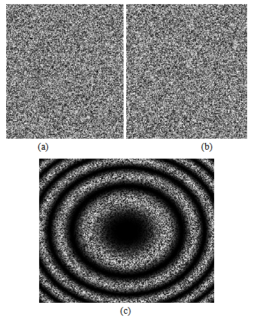 | Figure 2. (a) The primary interfergram, (b) the secondary interferogram, (c) the correlogram |
The intensity distribution in the primary interferogram (Fig.2.a) is given by: | (1) |
With  and
and  being the average intensity and the amplitude of the fringes respectively and
  is the speckle phase given by:
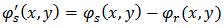 | (2) |
Such as  and
and  are the speckle phase and the reference speckle phase respectively.The intensity distribution in the secondary interferogram (Fig.2.b) is:
 | (3) |
 being the variation phase introduced by deformation.The intensity distribution in the correlogram (Fig.2.c) is:
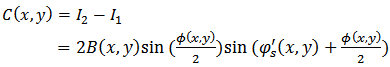 | (4) |
In this equation the phase of the deformation appears in the first term as an envelope modulating the speckle in the second term that varies spatially faster and can be removed by an appropriate filter.
3. Hilbert Huang Transform
3.1. The Empirical Mode Decomposition
The Hilbert-Huang transform (HHT) is based on the combination of the EMD method and the Hilbert transform (HT).The starting point of the Empirical Mode Decomposition (EMD) [5] is to consider oscillations in signals at a very local level. In fact, if we look at the evolution of a signal  between two consecutive extrema (say, two minima occurring at times
  and
and  ), we can heuristically define a (local) high frequency part
  , or local detail, which corresponds to the oscillation terminating at the two minima and passing through the maximum which necessarily exists between them. For the picture to be complete, one still has to identify the corresponding (local) low-frequency part
  , or local trend, so that we have
  for
for  .Assuming that this is done in some proper way for all the oscillations composing the entire signal, the procedure can then be applied on the residual consisting of all local trends, and constitutive components of a signal can therefore be iteratively extracted.Given a signal
  , the effective algorithm of EMD can be summarized as follows [5]:1. identify all extrema of
  2. interpolate between minima (resp. maxima), ending up with some envelope
  3. compute the mean
  4. extract the detail
  5. iterate on the residual
  In practice, the above procedure has to be refined by a sifting process [5] which amounts to first iterating steps 1 to 4 upon the detail signal d(t), until this latter can be considered as zero-mean according to some stopping criterion.
 | Figure 3. The BIMFs resulting from BEMD decomposition of the filtred correlogram |
Once this is achieved, the detail is referred to as an Intrinsic Mode Function (IMF), the corresponding residual is computed and step 5 applies. By construction, the number of extrema is decreased when going from one residual to the next, and the whole decomposition is guaranteed to be completed with a finite number of modes.
3.2. The Bidimensional Empirical Mode Decomposition
The BEMD permits to analyze a 2D non-linear and non-stationary data. Its principle is to decompose adaptively a given signal into frequency components, called Bidimensional Intrinsic Mode Functions (BIMF). These components are obtained from the signal by means of an algorithm called sifting process [6]. This algorithm extracts locally for each mode the highest frequency oscillations out of original signal.To extract the BIMF during the sifting process, we have used morphological reconstruction to detect the image extrema and RBF (Radial Basis function) to compute the surface interpolation. The bidimensional sifting process is defined as follow:* Identify the extrema (both maxima and minima) of the image I by morphological reconstruction based on geodesic operators;* Generate the 2D ‘envelope’ by connecting maxima points (respectively, minima points) with a RBF;* Determine the local mean m1; by averaging the two envelopes;*Since BIMF should have zero local mean, subtract out the mean from the image:  * Repeat as h1 is a BIMF.Adding all the BIMFs together with the residue reconstructs the original signal without information loss or distortion [7].
 | (5) |
The Fig.3 bellow represents the BIMF(i) of the filtred correlogram (Fig.6) to x=128 and i=1,4,7,10,13,16.
3.3. Hilbert Transform
In the real space, the Hilbert transform (HT) of the signal f(x) is a convolution between it and  [8]. It is defined by
 | (6) |
In the frequency domain, the Hilbert Transform results from a simple multiplication with the sign function: | (7) |
Where FT denotes the Fourier Transform, k is the angular frequency and | (8) |
The Hilbert transform does not change the amplitude F (k), it only changes the phase.Hence the Hilbert transform is equivalent to a filter altering the phases of the frequency components by 90° positively or negatively according to the sign of frequency.However, the direct application of this transform to a correlogram to carry out the phase shift sometimes introduces a sign ambiguity problem can be corrected by a guided method of fringe orientation correlogram [9].
4. Spatial Carrier Superposition
Owing to the difficulties encountered while experimentally adding the spatial carrier, we propose to add the spatial carrier to a fringe pattern numerically using the cosine fringe pattern and its  phase shifted version or sine fringe pattern [10].The fringe pattern of Eq. (4), leads after processing to a modulated fringe pattern which can be represented as follows
 | (9) |
After removing the background  by a high pass filter and applying the Hilbert Huang Transform, the resultant fringe patterns are:
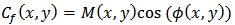 | (10) |
 | (11) |
Using a modulation ratio m, we numerically combine  and
and  with
with  and
and  giving the modulated fringe pattern:
 | (12) |
 | (13) |
A phase-modulated carrier my is then added to the phase of interest in order to enable the wavelet phase extraction lately.
5. Fringe Pattern Demodulation Problem
5.1. Principe
Fringe patterns analysis methods have been widely used to measure a wide range of physical quantities, modulated by a spatial phase, including surface profile and deformation, strain and temperature gradient. Consequently, phase retrieval becomes a key technique in the fringe pattern analysis field. The phase can be obtained from this fringe pattern by several methods including the Fourier and CWT (continuous Wavelet Transform) ones.
5.2. The Fourier Method
The Eq.9 can be written as: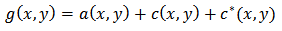 | (14) |
with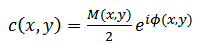 | (15) |
Where  is the conjugate complex of
  .It is possible to isolate the term
  , containing the phase information, in the frequency domain.The one-dimensional Fourier Transform, of Eq.14 has the following form:
 | (16) |
As the terms C and C* are symmetric, a filter containing only the positives frequencies has to be used to keep only the term  . Using the inverse FFT is needed to obtain
  that the
  modulus phase will be extracted from it as follow:
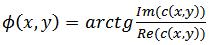 | (17) |
Notice that the phase needs to be appropriately unwrapped.
5.3. Wavelet Method
5.3.1. Continuous Wavelet Transform
The continuous wavelet transform (CWT) is a powerful tool to obtain a space–frequency description of a signal. Unlike the Fourier transform that uses an infinitely oscillating terms  , the wavelet analysis technique use a set of a specially designed pulse functions, called "wavelets", to analyze the local information of the signal [11]. A wavelet is an oscillating function
  , centered at x=0 and decay to zero such
  | (18) |
If  is the Fourier Transform of
  , then condition (18) is equivalent to the requirement that
  | (19) |
A family of the analyzing wavelets is generated from this “mother wavelet”  by translations and dilatations and it can be expressed as
  | (20) |
Where  is the scale parameter related to the frequency concept, and
  is the shift parameter related to position.We note that the wavelets with small values of s have narrow spatial support and consequently rapid oscillations, making them well adapted to selecting high-frequency components of a signal. The converse is true for wavelets with large values of s.Many different types of mother wavelets are available for the phase evaluation applications, but in our case the study reveals that the Complex Morlet wavelet gives the best results. It is defined as:
 | (21) |
Where  is the wavelet center frequency.Fig.4 shows the real and the imaginary part of the complex Paul wavelet.
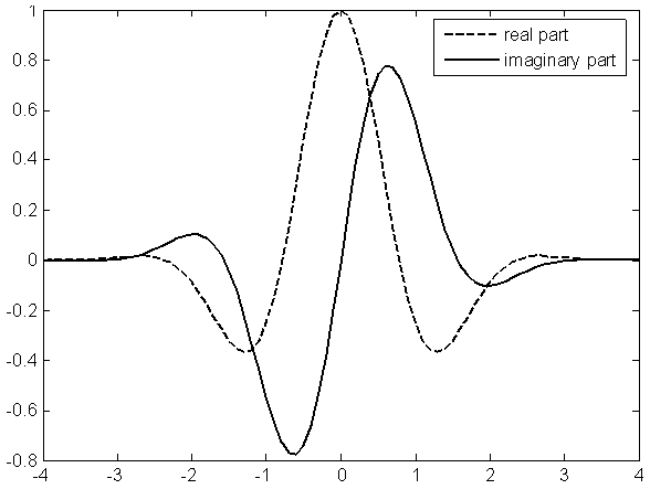 | Figure 4. Complex Morlet wavelet |
The 1D continuous wavelet transform (CWT) of a function  is giving by
 | (22) |
Where * denotes the complex conjugation.The continuous wavelet transform can be expressed, using the Parseval identity, as 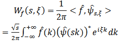 | (23) |
Where  ,
,  and
and  are the Fourier transform of the signal, the Fourier transform of the mother wavelet and the angular frequency,respectively. If the inverse wavelet transform exist, the original signal can be reconstructed by
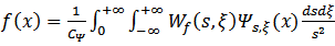 | (24) |
Where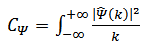 | (25) |
This reconstruction of the signal is possible when  has a finite value. The extension of the wavelet concept to the two-dimensional space is immediate by varying the integration variables and the location parameter in
  and neither in
  [12]. The 2D CWT of a two-dimensional signal f is given by
  | (26) |
where 
5.3.2. The 2D Wavelet-based Phase Retrieval Algorithm
To retrieve the phase information using the 2D wavelet method, the 2D CWT of the fringe pattern is computed by: | (27) |
Where 
 designates the orientation matrix by the angle
  :
: | (28) |
Thus the analyzing wavelets are resulted from the mother wavelet by dilatation, translation and also orientation processes [13].The wavelet coefficients array  is a 4D complex matrix that quantifies the local resemblance degree between the fringe pattern and the two-dimensional wavelet for different values of scale, location and orientation [14]. For each pixel, 2D wavelet coefficients matrix represents the directional structure of the fringe pattern. These coefficients capture the spatial dependence between the analyzing wavelet and the fringe pattern in different directions and for the specified frequencies. Thus, 2D wavelet transform proves to be very effective for retrieving the phase distribution in optical metrology.The wavelet coefficients, for the same location parameter values
  , form a 2D complex array
  that will be used to compute the phase of the fringe pattern pixel with coordinates
  .First, the ridge of the wavelet coefficients array
  is detected and the phase value will be its corresponding angle.
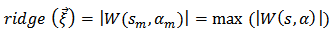 | (29) |
Where  and
and  are the scale and orientation values for maxima.
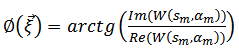 | (30) |
By repeating this process to all pixels of the fringe pattern, the phase map is then estimated. Notice that the resulted phase needs to be unwrapped via an appropriate algorithm to avoid spatial discontinuities.
6. Results and Discussion
The numerical simulation consists in generating digitally fringe patterns to verify the ability of the method to determine the phase distribution. The test phase function (Fig.5) that we used is expressed as: | (31) |
Where (x,y) are the pixel coordinates. | Figure 5. Simulated phase distribution. |
The fringe pattern shown in fig.2.c is the speckle correlogram coded by the known phase  .After filtering it by SWT filter [15], we obtained the resultant fringe pattern of Fig.6.
 | Figure 6. The filtered correlation fringes |
Using the BEMD decomposition, the first eight BIMFs of the fringe pattern are illustrated in Fig.7.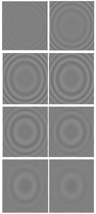 | Figure 7. The eight BIMFs components |
 | Figure 8. The  phase shifted correlogram phase shifted correlogram |
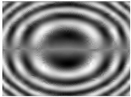
After that, the Hilbert Transform is applied to each BIMF followed by a sign correction. Fig.8 shows the sum of all corrected BIMFs. It’s a  phase shifted correlogram.After combining the two phase shifted fringe patterns numerically with sin (my) and cos (my), we have obtained the modulated fringe pattern shown in Fig. 9 with modulation rate value 0.8 radian/pixel.
 | Figure 9. The carrier fringe pattern |
The wavelet method was applied to the new carrier fringe pattern to retrieve the phase map of Fig. 10.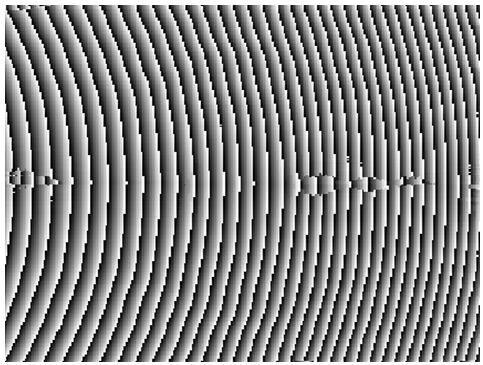 | Figure 10. The wrapped phase map |
Fig.11 illustrates the retrieved continuous phase map after the unwrapping process.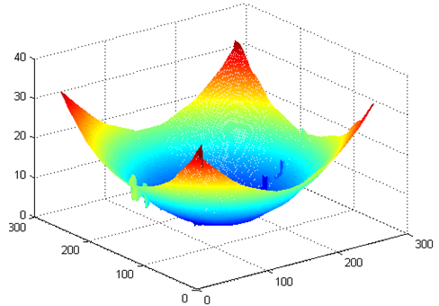 | Figure 11. The retrieved phase map |
Considering the structural Similarity index (measuring the similarity of the theoretical and retrieved phases) to evaluate the accuracy of the resultant phase, we obtained SSIM=0.87. The comparison of our algorithm is carried out with the Fourier phase retrieval method that was applied to an originally carrier fringe pattern coded by the same phase. The intensity of the carrier correlogram has the following expression: | (32) |
After applying the Fourier method on the new correlogram, the obtained phase distribution is displayed in Fig.12.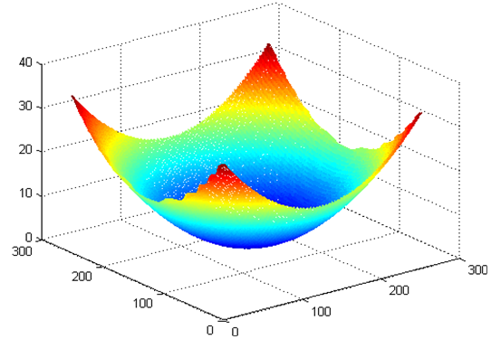 | Figure 12. The retrieved phase map by Fourier Transform |
The new Structural Similarity index that is obtained for Fourier method is 0.86.
7. Conclusions
In this paper, we have presented a new algorithm of phase retrieval from a single uncarrier corellogram with closed fringes. This was achieved by numerical superposition of the spatial carrier by Hilbert Huang Transform, followed by fringes demodulation using 2D Continuous Wavelet Transform.The use of the Bidimensional Empirical Mode Decomposition, before the  phase shifting by Hilbert Transform, helps to overcome the problem of the signal stationarity and frequency stability and helps to get a consistent and stable quadrature.The comparison of our algorithm to the well know Fourier method using an original carrier correlogram has shown that the results are in very close agreement with the advantage that our method is more suitable to the fast dynamic tests.
References
| [1] | Creath K. Phase-shifting speckle interferometry. Appl Opt 1985;24(18):3053–8. |
| [2] | Nakadate S, Saito H. Fringe scanning speckle-pattern interferometry. Appl Opt 1985; 24(18):2172–80. |
| [3] | R. Jones and C. Wykes, Holographic and Speckle Interferomertry, 2nd ed. (Cambridge U.Press, Cambridge England, 1989). |
| [4] | J.W.Goodeman; “Laser speckle and related Phenomena »; Vol.9 of Topics in Applied Physics (Springer-Verlag, Berlin, 1975). |
| [5] | N.E. Huang, Z. Shen, S.R. Long, M.L. Wu, H.H. Shih, Q. Zheng, N.C. Yen, C.C. Tung and H.H. Liu, “The empirical mode decomposition and Hilbert spectrum for nonlinear and nonstationary time series analysis,” Proc. Roy. Soc.London A, Vol. 454, pp. 903–995, 1998. |
| [6] | J.C. Nunes, Y. Bouaoune, E. Dele´chelle, S. Guyot, Ph. Bunel, Texture analysis based on the bidimensional empirical mode decomposition, Mach. Vision Appl. (2003) in press. |
| [7] | G. Rilling, P. Flandrin, and P. Goncalves, “On empirical mode decomposition and its algorithms,” in Proceedings of IEEEEURASIP Workshop on Nonlinear Signal and Image Processing, 2003. |
| [8] | Saff E. B., Snider A. D., Complex analysis for mathematics, science and engineering, Prentice- Hall, Inc., New York, 1976. |
| [9] | M Bahich, M Afifi, EM Barj, “Optical phase extraction algorithm based on the continuous wavelet and the Hilbert transforms”, Journal Of Computing, vol.2, 5, (2010). |
| [10] | E.M. Barj, et al., A digital spatial carrier for wavelet phase extraction, Optik 116 (2005) 507–510. |
| [11] | G. Kaiser; “A Friendly Guide to Wavelets”; (Birkhauser, Boston,Mass., 1994). |
| [12] | Mustapha Bahich , A comparative study of one and two-dimensional wavelet-based techniques for noisy fringe patterns analysis, Optics Communications 290 (2013) 43–48. |
| [13] | Mustapha Bahich,’ A numerical spatial carrier for single fringe pattern analysis algorithm’; Optik 122 (2011) 1821– 1824. |
| [14] | A. Abid, M. Gdeisat, D. Burton, M. Lalor, F. Lilley, Applied Optics 46 (2007) 6120. |
| [15] | E.M. Barj, et al., Speckle correlation fringes denoising using stationary wavelet transform. Application in the wavelet phase evaluation technique, Optics & Laser Technology 38 (2006) 506–511. |
 Abstract
 Reference
 Full-Text PDF
 Full-text HTML