1. Introduction

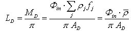
The integrating sphere has a relevant role in optics as it can be used as a light source with constant radiance or as a linear device for radiation measurements[1]. The integrating sphere has been widely used by us for the optical characterization of photovoltaic materials and devices and for radiation measurements on concentrated solar beams [2-17].

The theory of radiation emitted by an illuminated integrating sphere brings to the definition of the so called “sphere multiplier” M, a parameter which accounts for the increase of radiance, due to the internal multiple reflections, with respect to a planar diffuser with the same surface area. In what follows, we refer to the theory of integrating sphere as reported in refs.[18-21]. In this theory, the radiance L_D of a planar diffuser of total area A_D, without openings, and reflectivity ρ:

(1)

is compared to the radiance L_S of an integrating sphere of total area A_S = A_D , provided with openings for the input and output of radiation:

(2)

where f is the fraction area of openings. In the same theory, the first factor of second member of Eq. (2) is declared“approximately equal” to Eq. (1):

(3)

from which it is derived that the second factor of second member of Eq. (2) can be referred to the “sphere multiplier”:

(4)

We think that the equality (3) is incorrect and that it is possible to make a more precise treatment to define the “sphere multiplier”.

2. Alternative Definitions of “Sphere Multiplier”

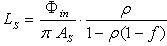
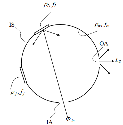
To make a correct comparison between the integrating sphere and the corresponding planar diffuser, we fix the same area in both cases and imagine that the integrating sphere surface be unfolded to realize the planar surface of the diffuser. Let us consider at first the simple case of a sphere of total area A_S, composed of an optically uniform wall surface and some ports with zero reflectivity for the input and output of radiation. The unfolded sphere gives rise to a planar diffuser (d) of total area A_D = A_S and some openings of area A_F = f · A_S (see Figure 1) where f is the fraction of openings area. If the surface has ideal diffusing properties, that is has a Lambertian behaviour, then the radiance L_D (W m^-2 sr^-1) of the planar diffuser is constant with viewing direction and can be expressed as follows:

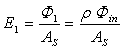
(5)

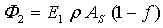
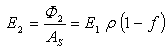
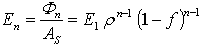
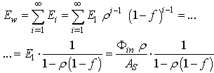
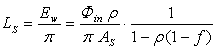
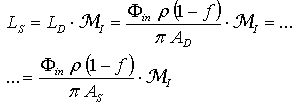
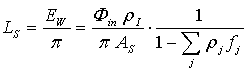
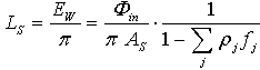
where M_D (W m^-2) is the exitance of the diffuser, Φ _in (W) is the flux impinging on the diffuser with reflectivity ρ and is the average reflectivity of the diffuser.

To calculate the radiance L_S of the integrating sphere (is), we refer to Figure 2. The (is) is irradiated by a collimated beam with the same flux Φ_in as before, entering the sphere through the input aperture (IA) and impinging on a small region (first impact region) of the internal wall. The radiance L_S is that measured from the radiation emitted by the output aperture (oa) of the sphere, and is obtained by the irradiance E_W produced on the internal wall at the stationary state, following the relation:

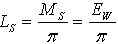(6)

where M_S is the exitance of the integrating sphere.

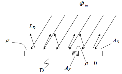Figure 1. A planar diffuser (D), with total area AD and wall surface with reflectivity ρ and fraction area f , is irradiated by the flux Φin and produces by reflection a flux with radiance LD at output

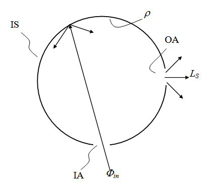Figure 2. The integrating sphere (IS) is irradiated by the flux Φin at input port (IA) and produces a flux with constant radiance LS at output port (OA)

To calculate E_W, let us consider the successive irradiance contributions produced on the wall by the multiple reflections. The first flux Φ₁ diffused into the sphere after reflection on the first impact region is:

(7)

This flux produces an irradiance E₁ on the sphere surface given by:

(8)

A new flux Φ₂ is produced into the sphere due to the second reflection:

(9)

Again we have an added irradiance component E₂ on the sphere surface:

(10)

and so on.

After the n-th reflection we have for the E_n component of irradiance:

(11)

At the stationary state we have for the total irradiance E_w:

(12)

By eqs. (6) and (12) we obtain for the radiance of the sphere:

(13)

The radiance of the sphere can be expressed as the product of the radiance L_D of the diffuser and the sphere multiplier M _I :

(14)

From eqs. (13) and (14) we obtain for the sphere multiplier M _I :

(15)

As it can be seen, our definition of sphere multiplier differs from that of Eq. (4), reported in refs.[18-20], being higher of the factor:[(1- f ) ·ρ]^-1.

Eq. (15) applies to a sphere realized with a wall with uniform reflectivity ρ and openings with fraction area f and zero reflectivity. In the general case, the sphere will be composed of, besides the wall, other different parts, like ports, detectors and other reflective surfaces, each of them characterized by a fraction area f_j and a reflectivity ρ_j (see Figure 3).

The unfolded sphere gives rise to a diffuser with radiance:

(16)

where is the average reflectance of the diffuser and of the sphere.

As regards the integrating sphere, we distinguish the first impact region, of fraction area f_I and reflectivity ρ_I, from the other portions of the sphere surface. Equation (8) becomes:

(17)

and Eq. (13) is modified as follows:

Figure 3. In the general case, the integrating sphere (IS) is not optically homogeneous. The generic part has reflectivity ρ j and fraction area f j . In particular, the first impact region is characterized by ρI and fI parameters and the wall surface by ρ w and f w parameters

(18)

By expressing the sphere radiance as the product of the diffuser radiance and the sphere multiplier, we have:

(19)

From Eq.s (18) and (19) we finally obtain for the general expression of the sphere multiplier:

(20)

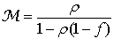
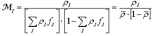
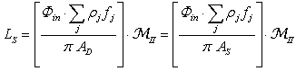
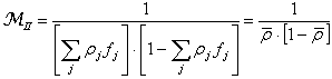
It is easy to verify that the general Eq. (20) becomes the simplified Eq. (15) when putting and 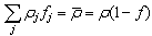, being ρ the reflectivity of the sphere wall. Eq.s (16), (18) and (20) are strictly valid in the hypothesis that all the portions of the sphere have a Lambertian behavior. In practice, this is well satisfied by the high reflectivity wall surface, less well by the surface of the accessories faced to the sphere interior.

In this paper we want to introduce a new definition of sphere multiplier, indicated as M_II. Considering the way how the planar diffuser and the integrating sphere are illuminated in the so far discussed approach, in fact, we note that the surface is uniformly illuminated by the input beam in the first device, whereas the input beam illuminates only the first impact region in the second one. To make a more congruent comparison between the radiance of the two devices, therefore, we should compare the diffused flux incident on the planar diffuser with the diffused flux produced into the integrating sphere after the first reflection. 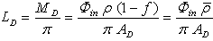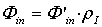In this new point of view, instead of putting equal the flux at input in the two devices, we put equal the diffused flux incident on the diffuser with the diffused flux incident on the integrating sphere wall surface soon after the reflection on the first impact region. We change, therefore, the flux at input of the sphere in order to have as the first diffused flux on the total area :

(21)

Now we can write for E₁:

(22)

and Eq. (18) is modified as follows:

(23)

By expressing the sphere radiance as the product of the diffuser radiance and the new sphere multiplier M_II :

(24)

we obtain for the new sphere multiplier:

(25)

For a simple sphere with only opening ports with fraction area f, Eq. (25) becomes:

(26)

Eq.s (25) and (26) represent, in our opinion, another valid definition of the sphere multiplier, as it comes from a comparison between a planar diffuser and an integrating sphere for which:

i) the area of the diffuser and of the sphere are exactly the same;

ii) the diffused flux at input incident on the diffuser surface and on the integrating sphere surface are equal.

3. Optical Simulations

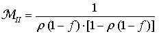
To highlight the difference between the new definitions of sphere multiplier, expressed by Eq.s (15), (20), (25) and (26), and the old definition expressed by Eq. (4), some optical simulations have been carried out taking into account realistic values for the optical parameters of the sphere. We consider a simple sphere composed of a homogeneous inner wall with reflectivity ρ and some windows for the input and output of the light, covering altogether a fraction area equal to f . These two parameters are sufficient to apply Eq.s (4), (15) and (26) for calculating the three sphere multipliers.

Figure 4 shows the sphere multipliers M, M_I and M_II calculated as a function of the reflectivity ρ , varying in the 0.9-1.0 interval, for three different values of the fraction area f : 0.01, 0.025 and 0.04. The value f = 0.04 is the maximum tolerated for assuring an optimal integration of light inside the sphere[19]. The reflectivity scale was extended to 1.00, but this is just a theoretical limit, not reachable in practice, as the best values of ρfor lambertian mirrors are around 0.99[19-21]. Figure 4 shows that for f = 0.01 the multipliers reach values as high as 50, and well higher values can be reached further reducing f. It is interesting to note the strong effect that the parameter f produces on the multipliers at high values of ρ. From Eq.s (4), (15) and (26), in fact, we can note that, in the limit ρ= 1, the multipliers depend only on f; in particular, M converges to 1/f, while M_I and M_II converge to 1/[f(1-f)], which are very close each other for very small values of f. A minor effect is instead produced by the different definitions of M. This effect is best appreciated by exploring lower values of ρ, as reported in Figure 5, where the three multipliers are shown for f = 0.01 and 0.04 as function of reflectivity ρ varying in the 0.8-0.95 interval. From Figure 5 we see that all the three multipliers tend to be less dependent on f at decreasing ρ in the examined, realistic range for the wall reflectivity of an integrating sphere.

We see also that the old multiplier M shows the lowest values, the new multiplier M_II shows the highest ones, and finally the new multiplier M_I shows intermediate values between them. Both the new definitions of sphere multiplier, therefore, determine improved values over the old definition. The multiplier M_II is 1/ρ times M_I , as established by Eq.s (15) and (26); this is due to the fact that the definition of M_I requires one more reflection on the wall, that one of the collimated beam at input, to produce the same diffused flux which is considered as input flux for the definition of M_II . This explains why the two quantities converge to the same value when ρ approaches the unity. Contrary to what may seem from Figure 5, the three multipliers tend to very different limits when ρ tends to zero. This is shown in Figure 6. For low values of ρ , M, M_I and M_II , go as ρ , (1+f) and 1/ρ , respectively. The examination of the range of low values of ρ is only speculative, since in practice the values of wall reflectivity in an integrating sphere vary in the range 0.8-0.99, depending on the fabrication process of the coating.

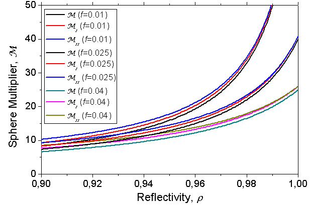Figure 4. Sphere multipliers M, MI and MII calculated as a function of reflectivity ρ in the 0.9-1.0 interval, for three different values of fraction area: f = 0.01, 0.025 and 0.04. The values obtained for ρ >0.99 are purely theoretical

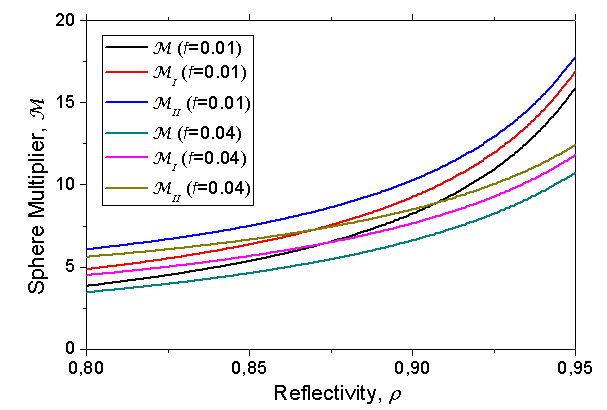Figure 5. Sphere multipliers M, MI and MII calculated as function of reflectivity ρ in the 0.8-0.95 interval, for fraction areas f = 0.01 and 0.04

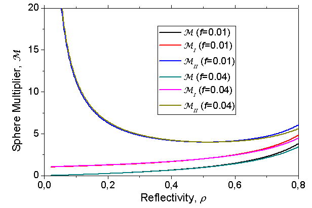Figure 6. Sphere multipliers M, MI and MII calculated for wall reflectivity in the 0.0-0.8 interval, for fraction areas f = 0.01 and 0.04

4. Conclusions

In conclusion, we have revisited the common definition of sphere multiplier distinguishing between two types of sphere multipliers, which differ only for the factor ρ_I. (reflectivity of the first impact region). The two multipliers have been defined considering the following different points of view:

i) M_I is obtained considering the same flux Φ_in at input of the planar diffuser and of the integrating sphere;

ii) M_II is obtained considering a different flux at input, but the same diffused flux at input on the total surface area of the two devices.

Differently from the actual theory, moreover, in our theory we have compared an integrating sphere, provided with the different openings for input and output of radiation and for radiation measurements, with a planar diffuser equal to the sphere in that it has been obtained by simply unfolding on a plane the sphere surface.

We have finally performed some optical simulations to compare the different definitions of multipliers for a simple geometry of the sphere, in order to highlight the influence of wall reflectivity and fraction area of the windows.