1. Introduction

Solar concentrators (SC) are usually investigated in order to know their optical transmission properties when they are irradiated by a uniform, collimated light beam simulating the direct component of the real solar radiation[1-6]. The most important result of this study is the curve of optical transmission efficiency drawn as function of the angle of incidence of the collimated beam respect to the optical axis of the concentrator (see Figure 1). The transmission curve is characterized by an acceptance angle, , corresponding to the 50% of the efficiency measured at 0°. This is valid for generic applications, whereas, for photovoltaic applications, an acceptance angle, , corresponding to the 90% of the efficiency measured at 0°, is usually adopted[7-10]. The other important property which is largely investigated in a solar concentrator is the spatial or angular distribution of the flux on the receiver, of minor importance in thermal solar concentrators, but of crucial importance in photovoltaic solar concentrators[11,12].

The optical transmission curve establishes how much precise must be the solar tracker, which brings the SC, when pointing towards the sun disk, in order to keep always the efficiency on the top of the curve[13], whereas the flux density distribution establishes if the system is suitable for the thermal or photovoltaic receiver, or if a secondary optical element (SOE) has to be added to it[14,15]. These are the basic information which are generally pursued, both theoretically or experimentally, by the people working on solar concentrators.

In this paper we try to go beyond this view by proposing a new scenario in which a solar concentrator, regardless of the type, if 2-D or 3-D, if refractive or reflective, if imaging or nonimaging, is studied as a generic optical component for which reflection, absorption or transmission properties can be defined respect to specific models of irradiation. We can distinguish, for example, between “direct” and “inverse” irradiation depending on the direction of the incoming light, or between “local” and “integral” irradiation depending if the irradiation is limited to a point or a small area of the aperture, or if it is extended to the entire aperture area; we can finally distinguish between a quasi-collimated irradiation by a far light source, in contrast to a “diffuse” irradiation by a lambertian source. In the last case we speak of a “lambertian” irradiation, understood as an irradiation with constant radiance from all directions within a maximum value of solid angle.

In what follows we talk about theoretical models of irradiation; these models are just simplifications of the real irradiation conditions which can be found outdoors. For each model we derive a specific method of characterization of the SC, that can be applied by optical simulations at a computer or by experimental measurements. The acronym assigned to each model of irradiation is the same of that assigned to the corresponding method of characterization.

In what follows a generic solar concentrator is schematised as a device confined between an entrance aperture (ia) with area A_in and an exit aperture (oa) with area A_out, where A_in > A_out , as the definition of solar concentrator requires. A solar concentrator operates in practice under “direct” irradiation, that is under irradiation on the entrance aperture and with a receiver, the energy conversion device, at the exit aperture.

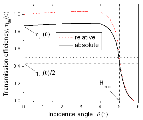Figure 1. Typical optical transmission curve of a nonimaging solar concentrator

In our models, however, we imagine to replace the receiver by any detector suitable to measure the total output flux, or its spatial and angular distribution; we imagine also to use the exit aperture to put there any source of light for inverse irradiation. The same considerations are valid when we consider the input aperture of the SC; we can measure the total flux exiting from it in reverse direction and its spatial and angular distribution and we imagine also to use the entrance aperture to put there any source of light for direct irradiation. What is there between the two apertures is specific of a particular fabrication technology and will not be considered here because it is not relevant, in principle, for a general discussion on its overall optical properties.

As the main question relative to the operation of a solar concentrator is its ability to transfer light to the output (here with light we intend the full spectrum of the sunlight or any portion of it), the simplest question to ask is: how an elementary beam, incident on (ia) at the point P(x, y) from direction, is transmitted by the concentrator? This question introduces the first and simplest method of characterization of the solar concentrator: the “Direct Local Collimated Method” (DLCM)[16-18]. To apply this method in the most general form we should consider also the polarization of the beam and its spectrum. In what follows, however, we simplify our discussion by considering always unpolarized and monochromatic light at input. The role played by unpolarized light, in fact, has a significant importance in this work. On the one hand a solar concentrator works mainly with direct sunlight, which is strictly unpolarized, on the other one, in the following, all the presented methods of SC characterization require the use of unpolarized light.

With the DLCM irradiation the elemental collimated beam is transmitted to output with an efficiency expressed by the quantity , the local optical transmission efficiency. When the test of the SC is performed on areas larger than the elementary area dA_in around the point P of the input aperture (ia), we are able, for example, to check the equivalence of symmetric portions of the input area of a real SC. We talk in this way of efficiency of direct transmission from these areas as: .

If the irradiation of the SC by a collimated beam is extended to the entire area of input aperture, we talk about the “Direct Integral Collimated Method” (DICM) or simply the “Direct Collimated Method” (DCM) (hereafter we will remove the term “Integral”, considering it implicit, so we will add only the term “Local” when we are irradiating only a portion of the aperture)[18,19]. Figure 2 illustrates the DCM. Before describing it, as well as the other methods discussed in this work, it is necessary to go to an “ab initio” investigation of the SC under the irradiation of an elementary beam.

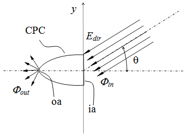Figure 2. Basic scheme of the Direct Collimated Method (DCM)

Figure 3 shows examples of the optical paths that an elementary beam can follow inside a SC, of refractive or reflective type, from (ia) to (oa) and vice versa. The beam can be totally reflected backwards (Figures 3e,f), or totally absorbed inside the concentrator (Figures 3g,h): these are extreme cases in which we cannot draw a path for light from the entrance to the exit aperture or vice versa. In all the other cases we can follow the beam from one aperture to the opposite one. We distinguish therefore between “connecting” and “not connecting” paths, when the paths connect or not the two apertures, respectively. Thus, we have connecting paths with direct irradiation in Figures 3a,d, and connecting paths with inverse irradiation in Figures 3b,c.

The attenuation that a light ray or an elementary beam experiments inside the SC is the result of all the interactions with the surfaces and the interfaces met during its travel. In the hypothesis that the beam undergoes only reversible processes[20], in particular reflections and/or refractions at planar surfaces, excluding surface diffusion or diffraction phenomena, the total attenuation of the beam can be derived by applying repeatedly the Fresnel equations. By indicating with the incidence angle and with the transmission angle (by reflection or refraction), it can be found, by Eqs. (1a) and (1b), that the transmission factors T_refl for reflection and T_refr for refraction do not change at exchanging and angles, that is inverting the direction of travel of the light path, as established by the “reversibility principle”: “the attenuation undergone by an unpolarized beam on the same path, but at opposite direction, is the same”.

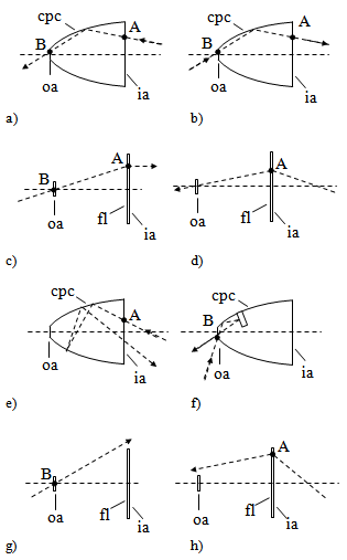Figure 3. Examples of “connecting” (a-d) and “not connecting” (e-h) light paths; (cpc): nonimaging concentrator, (fl): imaging Fresnel lens; beams: (a, d) direct transmitted; (b, c) inverse transmitted; (e) direct reflected; (f) inverse reflected; (g) inverse absorbed (h) direct absorbed

(1a)

(1b)

The rays back reflected or totally absorbed, that is the rays completely lost, have a transmission factor equal to zero and no "connecting" paths between the two apertures can be defined for them. The identical connecting paths, as A→B of Figure 3a and B→A of Figure 3b, have the same transmission factor: T_AB = T_BA, when the starting beam is unpolarized. When the methods described in the following are applied, the condition of depolarisation of incident beam must be accurately verified, both for the “direct” and the “inverse” sources.

The condition T_AB = T_BA is the basis of the so called “Inverse Lambertian Method” (ILM), which has been conceived for deriving the absolute transmission efficiency of DCM by analysing, instead of the flux collected at the receiver (the output aperture) with direct irradiation, the flux collected at input aperture with the inverse irradiation[21-25]. In order to apply this concept, it is necessary that the rays analysed with the “direct” irradiation overlap those analysed with the “inverse” irradiation, that is, that the respective optical paths be identical.

Now, in the direct irradiation by DCM, the input beam should be varied, in principle, in the 0°-90° range of polar angle. In order to deduce, therefore, the attenuation undergone by the direct rays inclined at any polar angle respect to the optical axis, it is necessary to analyse all the inverse rays emitted by the concentrator in any direction from the input aperture. The source of the inverse rays must be placed in correspondence of the receiver (the output aperture) and must be able to emit rays, from each point and in any direction inside the SC, at constant radiance, in order to not discriminate any direction. Only in this way it will be possible to produce, in the inverse mode, all the connecting paths which will overlap with those that are produced in direct mode by a collimated beam inclined at different polar angles between 0° and 90°. In order to apply the “inverse” method ILM in a correct way, therefore, we need to put a spatially uniform lambertian source at the output aperture, as shown in Figure 4a, where is the constant radiance of the inverse lambertian source.

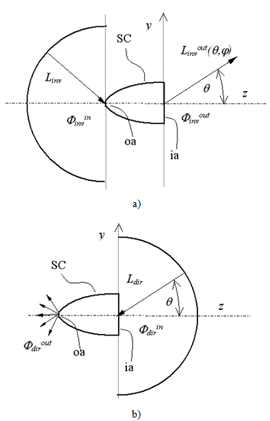Figure 4. a) Scheme of the “Inverse Lambertian Method” (ILM). b) Scheme of the “Direct Lambertian Method” (DLM). In both cases we consider a limit polar angle = 90°

If we want to analyse the SC, activating simultaneously all the connecting paths in direct mode, we should consider an infinity of beams impinging on the input aperture at different polar angles. This is achieved as well by using a spatially uniform lambertian source placed at the input aperture, as schematised in Figure 4b, where is the constant radiance of the direct lambertian source.

If the concentrator is irradiated simultaneously in “direct” and “inverse” modes by lambertian sources, all the connecting paths will overlap and, putting =, also the elementary flux flowing through any connecting path will be the same along the two directions. Then, with =, also the total flux flowing through the concentrator from one aperture to the other will be the same in the two directions. The irradiation of the SC by diffused lambertian sources introduces in this way the “lambertian” methods of irradiation, based on the irradiation with constant radiance from any direction: the “Direct Lambertian Method” (DLM) shown in Figure 4b with light incident on the input aperture[16,17,19,25], and the “Inverse Lambertian Method” (ILM) shown in Figure 4a with light incident on the output aperture[21-25]. In the following Section, the models briefly outlined so far will be investigated in detail.

2. Theoretical Models of Light Collection

2.1. Theory of the “Direct Collimated Methods”

An elementary beam, incident on the point A of (ia) and flowing inside the SC in the direct mode, (see Figures 3a, d), will be transmitted to the output with an efficiency ≤ 1. Alternatively, the elementary beam will be reflected backwards (Figure 3e) or totally absorbed inside SC (Figure 3h). In practice, the DLCM is easily applied by utilising a laser beam as it illustrated in[16-18]. If is averaged over a uniform distribution of points P on the input aperture, the transmission efficiency at collimated light of the SC can be approximately estimated[16]. The precise estimation of , however, requires the full irradiation of input aperture by a collimated and uniform light beam, and this is obtained by the application of the “Direct Collimated Method” (DCM), the most appropriate method to simulate the behaviour of a SC operating under the direct solar irradiation. As we have seen in the Introduction, the most important quantity summarizing the properties of light collection of a solar concentrator (SC) is its “absolute” transmission efficiency , expressed as function of the polar and azimuthal angles of direction of the collimated beam, characterized by a constant irradiance E_dir on the wave front (see Figure 2):

(2a)

where is the area of input aperture projected along direction . If the contour of input aperture is contained on a plane surface, Eq. (2a) simplifies as:

(2b)

The “absolute” transmission efficiency can be expressed as:

(3)

where is the “relative” transmission efficiency of the SC and is the transmission efficiency at 0° (see Figure 1). It is clear that is the average value of , the local, collimated optical efficiency, when is calculated for all the points of the entrance aperture. We have therefore for the output flux:

(4)

and for the transmission efficiency:

(5)

The basic scheme of the “direct collimated method” (DCM) is shown in Figure 2. The representation of a perfectly parallel beam, as in Figure 2, is purely ideal and cannot be achieved in practical experiments. The flux at input can be written in fact as:

(6)

To have a perfectly parallel beam, we should have = 0, that is should be infinite to have a finite flux at input, and this is impossible to reach in practice. In an ideal experiment, we could imagine collimating light from a dimensionless source placed in the focus of a parabolic mirror, or to collect light from a source of finite dimension placed at infinite distance: in both cases the radiance of the light source becomes infinite. So we can write more precisely for the direct optical efficiency under a collimated beam:

(7)

where is the radiance, from the direction, of a finite source at finite distance, and the symbol  is for “transmitted”.

To explore the full properties of light collection of the SC, the collimated beam must be oriented respect to the optical (z) axis of concentrator varying  in the 0°-90° interval and  in the 0°-360° interval. If the SC has cylindrical (rotational) symmetry, it is sufficient to fix a value and to vary only . Generally, the SCs have squared or hexagonal input apertures, because these geometries allow to pack better them in a concentrating module, then the angle can be limited, in these cases, to the 0°-90° or the 0°-60° interval, respectively. Despite this limitation, however, the number of measurements required by the application of DCM is very high, both for simulations and for experimental measurements. This is indeed the very strong limit of DCM applied to the determination of . This limit can be overcome by the use of the “Inverse Lambertian Method” (ILM) of irradiation, as it is demonstrated in Section 2.3.

Dealing with “nonimaging” SCs[1,2,26], whose transmission curve has a step-like profile (see Figure 1), their characterization by DCM can be simplified; it is sufficient in fact to vary the input angle from 0° to a little more than the acceptance angle at 50% of 0° efficiency, . The rays incident at , in fact, will be rejected back by the SC before reaching the output aperture.

The quantity (see Figure 1) represents the fraction of flux transferred to the output, and then it represents the “direct transmittance” at collimated light, or “direct collimated transmittance” of the SC, when it is viewed as a generic optical component. In like manner, we can speak of a “direct collimated reflectance” or of a “direct collimated absorptance” of the SC for the fraction back reflected or absorbed of the input flux, respectively:

(8)

(9)

We have for the conservation of energy:

(10)

We observe that, while the fraction of transmitted flux at output is generally measured, the reflected or absorbed ones are not; only the total lost flux is deduced from Eq. (10). The measure of is however possible in principle; it is a simple task by simulation (see the forthcoming parts of this work); more difficult it is to do it with experimental measurements.

A typical curve of for a 3-D nonimaging concentrator like a CPC (Compound Parabolic Concentrator) is illustrated in Figure 1[1,2,26]. Here the angle is not represented as the CPC has a cylindrical symmetry. We distinguish the 0° efficiency , the acceptance angle at 50% of 0° efficiency and the relative transmission curve , characterized by the same angle, as it can be easily demonstrated. Respect to solar concentrators like the nonimaging CPCs, the “imaging” solar concentrators show a very different transmission curve, with a long tail and a short flat portion at small angles[1]. For these concentrators the DCM has to be applied by varying the polar angles from 0° to a limit angle, , well higher than . The transmission curves or are defined for a perfectly collimated light and can be drawn easily by simulations with an optical code. With experimental measurements, however, the beam will be quasi-collimated, with a divergence angle which depends on the design of the apparatus, so the drawing of the curve in this case contains a margin of indetermination.

2.2. Theory of the “Direct Lambertian Methods”

The “Direct Lambertian Method” (DLM)[16,17,19,25] allows to study the transmission efficiency of a concentrator when the irradiation at input is integrated over all the directions in space. DLM simulates the behaviour of the concentrator under diffused light, for example the diffuse solar radiation in a totally covered sky. A clear sky, in fact, contrary to appearances, is not a good example of isotropic light, because the polarization of solar light by Rayleigh scattering produces a radiance strongly dependent on the direction of diffuse light respect to the direction of Sun[27]. Figure 4b shows the scheme of DLM applied to a 3D-CPC concentrator, with constant radiance of the diffused light source. The total incident flux is:

(11)

where is the étendue.

In the following, we will consider, for simplicity, only concentrators with cylindrical symmetry, then will be set equal to . The equations can be easily extended, whenever necessary, to the general case by reintroducing the dependence on the azimuthal angle . The flux “transmitted” to the output aperture becomes:

(12)

The optical losses due to the “reflected” flux and to the “absorbed” flux are expressed respectively as:

(13)

(14)

in such a way that: . Here is the “direct collimated reflectance” and is the “direct collimated absorptance” of the concentrator, as previously defined.

DLM gives the “direct lambertian transmission efficiency” , also called “direct lambertian transmittance” , defined as the ratio of output to input flux:

(15)

In a similar way we define the other two quantities related to DLM: the “direct lambertian reflectance”and the “direct lambertian absorptance” :

(16)

(17)

where: =1.

The output radiance, in general, is not constant like the input radiance, so we speak about an average output radiance:

(18)

where is the geometrical concentration ratio. Now we define a new quantity, , the ratio between output and input radiance:

(19)

From Eq.s (15), (19) we find the relationship:

(20)

Eq. (20) has the same form of the relationship defining the optical concentration ratio of a SC under collimated irradiation[1]:

(21)

We define therefore the quantity as the “optical concentration ratio under direct lambertian irradiation” or “direct lambertian concentration ratio”.

The direct lambertian model can be applied also reducing the angular extension of the lambertian source from π/2 to a limit polar angle (see Figure 5). The corresponding method, DLM, is particularly useful when we analyse the behaviour of nonimaging SCs. Because of the step-like profile of their optical efficiency (≈ 0 for ), in fact, the characterization of these SCs under direct lambertian irradiation can be limited to angles , reducing in this way the time of computer elaboration or simplifying the experimental measurements.

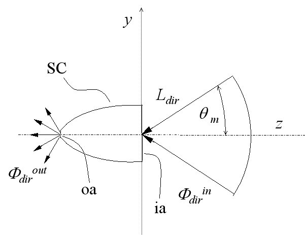Figure 5. Scheme of the “Direct Lambertian Method ”, DLM ()

The DLM can simulate the irradiation of a SC by a near lambertian light source, as illustrated in Figure 6. The theory of DLM is just that developed until now for the DLM, modified in the limit polar angle of the diffused irradiation. We have therefore for the input and output flux:

(22)

(23)

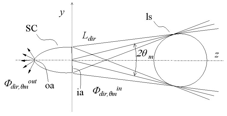Figure 6. Irradiation of the SC by a nearby lambertian source (ls)

The direct transmission efficiency of this method becomes:

(24)

The average output radiance becomes: :

(25)

and the optical concentration ratio is:

(26)

2.3. Theory of the “Inverse Lambertian Methods”

We saw in the Introduction that, for the reversibility principle, the optical loss reported by a direct ray is the same as that shown by an inverse ray if the optical path is the same and if both starting rays are unpolarized. The attenuation factor for the radiance of the direct beam incident at point A in direction represents the local direct transmission efficiency (see Figure 3a), while the attenuation factor for the radiance of the ray emitted by the SC from point A in the reverse direction (see Figure 3b) represents the local inverse transmission efficiency . We extend now these concepts to all points of directly irradiated in direction (DCM, see Figure 2) and to the same points of that emit light in the reverse direction (ILM, see Figure 4a). If the inverse radiance at output aperture (Figure 4a) is constant for all directions, that is, if the source at output aperture is Lambertian, then the inverse output radiance, , averaged over all points of , must have the same angular distribution of the inverse transmission efficiency , averaged over all points of . But the average inverse transmission efficiency must have the same angular distribution of the average direct transmission efficiency , because the transmission of the single connecting paths is invariant respect to the direction of travel of light. As a consequence, we can affirm that the inverse radiance of the concentrator , irradiated on the output aperture with a uniform and non-polarized Lambertian source, is proportional to the efficiency of the direct transmission of a non-polarized collimated beam, that is the two corresponding relative quantities coincide. We have therefore that:

(27)

where:

(28)

(29)

Eq. (27) establishes the equivalence between the “relative” inverse radiance and the “relative” direct transmission of the SC. The above discussion demonstrates therefore the suitability of the inverse lambertian method (ILM) to provide all information concerning the relative efficiency of transmission of the concentrator under direct irradiation, (see Figure 1).

The simulated and experimental measurements of relative inverse radiance of a solar concentrator is discussed elsewhere[21-25]. Here we recall that, to perform these measurements, it is sufficient to project the inverse light of concentrator towards a far planar screen and to record the image produced there; a simple elaboration of the image gives , and so .

Here we want to emphasize another fundamental aspect of ILM, that is the fact that it provides also the value of , and so the “absolute” transmission efficiency (see Eqs. (3), (29)), without recourse to any direct measure by DCM[24,25], as it will be demonstrated by the following considerations.

When the SC is irradiated in the reverse way (see Figure 4a), the exit aperture (oa) of area becomes a Lambertian source with constant and uniform radiance . The total flux, injected into the SC and function of radiance , becomes:

(30)

The inverse flux transmitted to output, the input aperture (ia) of area of the SC, is given by:

(31)

where is the radiance of light inversely emitted towards . We now define the inverse lambertian transmission efficiency, or “inverse lambertian transmittance”, , as the ratio of output to input flux:

(32)

Let us compare the inverse lambertian transmittance of Eq. (32) with the direct lambertian transmittance of Eq. (15) by taking their ratio:

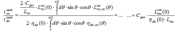(33)

This ratio is just a property of the SC and should not depend on radiance quantities as it appears in Eq. (33). To clarify this situation, we calculate the ratio by applying the simple condition = , at which the total integral flux transmitted in the “direct” and the “inverse” directions is the same: = , because such is the flux transmitted through the elementary connecting paths in the two directions. By putting = and using Eqs. (12) and (31) we find:

(34a)

Putting = and applying Eqs. (28), (29), we have:

(34b)

We finally find:

(34c)

Eq. (34c) tell us that we can calculate by ILM measuring , the average on-axis inverse radiance of SC, and , the radiance of the inverse lambertian source[24,25]. From Eq.s (33), (34c) we find moreover that the ratio between the inverse and direct lambertian transmittances is equal to , that is independent on radiance, as foreseen. This could be also deduced by considering that, if = , we have:

(35)

that is: the “inverse lambertian transmittance” of a SC is times its “direct lambertian transmittance”, or equivalently: the “input direct lambertian flux” needed to sustain an equal transmitted flux in the opposite directions is times the “input inverse lambertian flux”. This result is not surprising; it is a direct consequence of the geometrical asymmetry of the concentrator and disappears when =1, that is=. It is interesting to note that this result does not require any information about the internal features of the SC, but is only dependent on the sizes of the lateral apertures. Eq. (35) tell us that the optical “transparency” of the SC to lambertian light is not symmetric.

Let us imagine now to irradiate both apertures of the SC by two different lambertian sources with ≠ (see Figure 7). If is the difference of incidence radiance between input and output, then we have for the net flux through SC, in the direct direction:

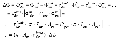(36)

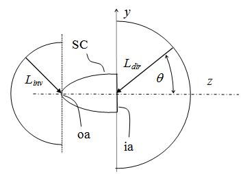Figure 7. Scheme of the irradiation of the SC by both “Direct Lambertian Method” (DLM) with radiance Ldir and “Inverse Lambertian Method” (ILM) with radiance Linv

From Eq. (36) we deduce, for example, that a CPC immersed in an integrating sphere has no net flux flowing through it (the radiance is constant inside the integrating sphere, so = 0). Eq. (36) has a strong similarity with the Ohm’s law:

, where (W) has the role of current, (W/sr·m²) the role of potential difference and (sr·m²) the role of conductance. The net flux inside the SC, indeed, is the natural optical partner of the electric current and the choice of the radiance as the optical partner of the electric potential is the only one which allows to put Eq. (36) in the form of the Ohm’s law. Attempts to assign the role of potential to the total input flux or to the étendue are in fact unsuccessful. From Eq. (36) we define the “direct conductance under lambertian irradiation” or “direct lambertian optical conductance” :

(37)

The surprising result is that, if we reverse the SC keeping fix the radiance gradient, now the flux flows in the inverse direction with the same conductance. We have in fact, changing the sign to both members of Eq. (36) and using Eq. (35):

(38)

with . From Eq. (38) we define the “inverse conductance under lambertian irradiation” or “inverse lambertian optical conductance” :

(39)

From Eqs. (37), (39) we conclude that the two conductances are equal:

(40)

The result of Eq. (40) is surprising in the fact that the optical asymmetry of the SC has disappeared as long as the conductance of the SC is considered. Eqs. (37) and (39) show that the “optical conductance” can be put in the form:

(41)

that is: “conductance” = “étendue” x “transmittance”. Now the equivalence between the two opposite conductances is direct consequence of the fact that the “direct” étendue is times the “inverse” étendue and that the “inverse” transmittance is times the “direct” transmittance.

From Eq. (36) we derive the density of the net flux through the input aperture (the average net flux flowing through the unit area of the input aperture inside the SC in direct way):

(42)

where .

and the density of the net flux through the output aperture (the average net flux flowing through the unit area of the output aperture inside the SC in the reverse way):

(43)

where .

If is the length of the SC, we can introduce the quantity , the average gradient of radiance through the concentrator, a quantity which cannot be measured in practice, but which can be imagined to exist inside the concentrator from a theoretical point of view. Eq. (42) becomes:

(44)

In Eq. (44) grad is intended as the average of the gradient of . Eq. (44) is optically equivalent to the Ohm’s law expressed in local form: , with (W/m²) with the role of current density, gradΔL (W/sr·m³) with the role of electric field and (sr·m) with the role of electrical conductivity. The equivalent expression for the inverse current density is given by:

(45)

We can define therefore a “direct lambertian optical conductivity” and an “inverse lambertian optical conductivity” of a solar concentrator as follows:

(46)

(47)

From Eqs. (46), (47) and (35) we see that:

(48)

The Eq. (48) tell us that the “inverse optical conductivity” of a SC is times its “direct optical conductivity”, so it restores the asymmetry of the concentrator, as we have found for the transmittance efficiency.

As we have seen for the direct local collimated method (DLCM), which applies only to a portion of input opening, the local inverse method can be applied fruitfully to small or large areas of the exit opening. We talk in this way of areas , and of efficiency of direct transmission to these areas as: . The efficiency can be obtained by applying the ILLM method to measurements of , when the receiver is inversely irradiated by a lambertian source placed in the area and centred on point P. The new situation is similar to that which would occur if the concentrator could be amended as follows: the new receiver is the selected area of the old receiver; the new concentrator is the old concentrator plus the excluded area of the receiver. This new way of looking at the receiver is very powerful. In this way, in fact, we can study the efficiency of collection of any portion of the optical receiver, and since the radiation on the receiver is generally not uniform when the concentrator is directly irradiated, it happens often to be wonder about the direction of the direct rays arriving in a certain area of the receiver. By applying the ILLM method, therefore, we can know from which direction the rays in excess in a certain area of the receiver arrive, or from which direction they are failing to arrive in a certain area of it. In a forthcoming part of this work, the applications of the ILLM method to nonimaging CPCs will be shown.

Recent developments of the “inverse lambertian method” have been proposed by Herrero et al.[30,31], which have shown that the method can be modified in a way suitable to use the solar cell as receiver in PV concentrators, and have proposed the use of a parabolic mirror to project the inverse light of concentrator towards the planar screen. In a subsequent work, Parretta et al.[32] have modified the Herrero method by extending the use of the parabolic mirror also for measurements on a generic SC (photovoltaic or thermodynamic).

3. Conclusions

In conclusion, we have presented in this work a general theoretical approach to the study of a solar concentrator looked at as a generic optical component. Irrespective of its practical way of use, we have considered any type of irradiation on the concentrator, and, for each type of irradiation, its reflection, absorption and transmission properties have been defined, both locally on its apertures and on its entire surface of its apertures. But, most importantly, the classical view of the concentrator fully irradiated on the front side by a collimated beam has been upset and a new way of looking to it has been introduced through the new concept of “inverse” irradiation. By inverting the irradiation of the concentrator and by using a lambertian distribution of light at the output, new and surprising results appear, which allow us, besides other things, to disclose the full direct optical transmission properties of the solar concentrator by a very simple approach. Besides this, we have been able to introduce new optical concepts and to define new optical quantities making similarities with electrical concepts. All the results have been obtained applying two optical concepts: the reversibility principle and the efficiency of transmission through the solar concentrator of an elemental beam.

In the forthcoming parts of this work the simulations and the experimental measurements pertaining to the presented methods will be discussed in detail, referring in particular to nonimaging solar concentrators (CPCs).