-
Paper Information
- Paper Submission
-
Journal Information
- About This Journal
- Editorial Board
- Current Issue
- Archive
- Author Guidelines
- Contact Us
Research in Neuroscience
2012; 1(2): 8-16
doi: 10.5923/j.neuroscience.20120102.01
Experimental Data Fitting Analysis on Frequency-Current-Temperature Relation
 Abstract
 Reference
 Full-Text PDF
 Full-Text HTML
Yasuomi D. Sato 1, 2, Chiaki Kobayashi 3, Yuji Ikegaya 3
1Department of Brain Science and Engineering, Graduate School of Life Science and Systems Engineering, Kyushu Institute of Technology, Kitakyushu, 808-0196, Japan
2Frankfurt Institute for Advanced Studies (FIAS), Goethe University Frankfurt, Frankfurt am Main, D60438, Germany
3Laboratory of Chemical Pharmacology, Graduate School of Pharmaceutical Sciences, the University of Tokyo, Tokyo, 113-0033, Japan
Correspondence to: Yasuomi D. Sato , Department of Brain Science and Engineering, Graduate School of Life Science and Systems Engineering, Kyushu Institute of Technology, Kitakyushu, 808-0196, Japan.
| Email: |  |
Copyright © 2012 Scientific & Academic Publishing. All Rights Reserved.
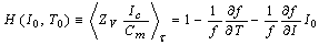
We study experimental data fitting to a frequency gradient curve for current and temperature simulated with the Hodgkin-Huxley (HH) oscillator undergoing saddle-node on invariant cycle bifurcation. In this study, one frequency gradient curve (referred to as the theoretical curve) are constructed by expanding the HH oscillator using small perturbations of the current and temperature while the other gradient curve (referred to as the empirical plot) is obtained with frequency-current relations recorded from hippocampal CA3 pyramidal cells at different environmental temperatures. The empirical plot is best-fitted to the theoretical curve under a certain temperature parameter range using simulations with the HH oscillator. In order to confirm the best-fit, we show that the theoretical curve is overlapped almost of the standard errors for the plot and that a temperature coefficient in the HH oscillator is rescaled to be in a suitable range of the temperature coefficient calculated with the experimental data.
Keywords: Frequency Gradient Curve, Cold-Receptor-Like Neuron, Saddle-Node Bifurcation on Invariant Cycle, Hodgkin-Huxley Model, Temperature Coefficient
Cite this paper: Yasuomi D. Sato , Chiaki Kobayashi , Yuji Ikegaya , "Experimental Data Fitting Analysis on Frequency-Current-Temperature Relation", Research in Neuroscience , Vol. 1 No. 2, 2012, pp. 8-16. doi: 10.5923/j.neuroscience.20120102.01.
Article Outline
1. Introduction
- Sensitivities for environmental temperature and body temperature are vital functions for creature as well as human beings. Thermosentive receptors or neurons, which seem to be broadly distributed on the skin and in the brain, are classified into two categories, those that sense warmth and those that sense cold[1],[2]. In particular, cold receptors are usually excited in the presence of a cold stimulus. Its activities paradoxically respond when the temperature is relatively high (for example, above 45℃ in the cold receptor on slowly conducting fibers[3]). Such activities were modelled with a Boltzmann description of voltage-gated membrane channels[4].Since the Boltzmann model does not differ functionally from standard Hodgkin-Huxley (HH) formulations[5], the Boltzman as well as HH models can be interpreted as models of detection of body temperature in the brain area. In fact, the HH model, which begins repetitive firings with zero frequency via a saddle-node bifurcation occurring on an invariant cycle (called the SNIC), shows the aforementioned spike activities dependent on temperature variations[6]. In[7], a frequency increase with a temperature Copyright © 2012 Scientific & Academic Publishing. All Rights Reservedreducti-on was calculated even with the Morris-Lecar (ML) model[8],[9], which has a common structure with two dimensional excitability models such as the (V, n)-reduced HH model[10]. This indicates that such an increase may be caused by nonlinearity of the main current dynamics. We thus suppose it meaningful to understand mechanisms on such temperature-dependent neuronal properties.It is also important to examine whether or not neurons sensing body temperature variations exist in the nervous system, for the sake of homeostasis or stabilities in brain functions. The brain functions have been well known to be affected by small changes in brain temperature (as little as 2-3℃)[11-13]. Effects of physiological body temperature on neural activities in the hippocampal slice have been more intensively studied since 2007, those being, regulation of resting membrane potentials[14], increased synchronized network activity[15] and increased frequency of γ-oscillation[16]. These experiments give us one of indications that cold-receptor-like neuronal activities may even be observed in the brain.The concrete target of this work is to analyze a frequency-current (f-I) curve that is V-shaped with a temperature (T) increase, recorded from pyramid cells in the hippocampal CA3 slices, indicating that the pyramidal cells may functionally act as cold neurons. For this target, the HH model exhibiting the SNIC bifurcation with an I increase is employed with the parameter sets as referred to[17]. We simulate that the HH model behaves like the cold receptor activation as mentioned above, calculating f at different T and different I values.Next, making phase descriptions for small perturbations of ΔI and ΔT within the framework of the phase reduction method[18-20], we derive the theoretical formulation of frequency gradients for I and T. The frequency gradient formulation gives us an explanation of how the theoretical curve for the HH model should best-fit to the empirical plots. In the most appropriate fittings, a temperature coefficient Q10 in the HH model is rescaled to the value that is in a good agreement with the empirical Q10 calculated by the experimental data. Finally, discussion and conclusion will be given.
2. Methods and Materials
2.1. Slice culture preparation
- Entorhinal-hippocampal organotypic slices were prepared from 7-d-old Wistar/ST rats. Rat pups were anesthetized by hypothermia and decapitated[21]. The brains were removed and placed in aerated ice-cold Gey’s balanced salt solution supplemented with 25 mM glucose. Horizontal entorhinal- hippocampal slices were cut at a thickness of 300 μm using a vibratome. The slices were placed on Omnipore membrane filters and incubated in 5% CO2 at 37℃. The culture medium, which was composed of 50% minimal essential medium, 25% Hanks’ balanced salt solution, 25% horse serum, and antibiotics, was changed every 3.5 d. The slices were cultured for 10-15 days in vitro and used for electrophysiological experiments.
2.2. Electrophysiology
- An entorhinal-hippocampal slice was placed in a recording chamber and perfused at 25, 30, and 35℃ at a rate of 3-4 ml/min with artificial cerebrospinal fluid (aCSF) consisting of 127 mM NaCl, 26 mM NaHCO3, 3.5 mM KCl, 1.24 mM KH2PO4, 1.0 mM MgSO4, 1.8-2.0 mM CaCl2, 10 mM glucose, 10 μM CNQX, and 50 μM AP5[22]. The temperature was controlled using an in-line heater (SC-20l, Warner instruments). For whole-cell recordings borosilicate glass pipettes (4-6 MO) were filled with solution consisting of 130 mM K-gluconate, 10 mM KCl, 10 mM HEPES, 10 mM phosphocreatine, 4 mM MgATP, 0.3 mM NaGTP. Data were obtained using a MultiClamp 700B amplifier and a Digidata 1440A digitizer controlled by pCLAMP 10 software (Molecular Devices). Signals were low-pass filtered at 2 kHz and digitized at 20 kHz.
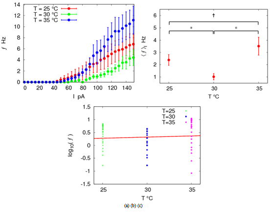 | Figure 1. Frequency (f Hz) is temperature-dependent. (a) f-I plots at 25, 30 and 35℃. (b) The average frequency over all I steps,  , is plotted at each temperature. P†< 0.01, compared with T = 25℃ sampling data, and P* < 0.001 (n = 6), compared with T = 30℃, ANOVA. (c) log(f)-T line results in the temperature coefficient Q10 = 1.22 ± 0.38 , is plotted at each temperature. P†< 0.01, compared with T = 25℃ sampling data, and P* < 0.001 (n = 6), compared with T = 30℃, ANOVA. (c) log(f)-T line results in the temperature coefficient Q10 = 1.22 ± 0.38 |
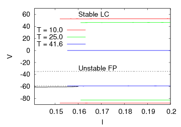 | Figure 2. Bifurcation diagram for the SNIC HH model when increasing temperature from 10, 25 to 41.6℃ for I = 0.161. The broken lines represent unstable fixed points (FP). One is the saddle while the other is focus. The solid lines represent stable focus and stable limit cycle (LC) |
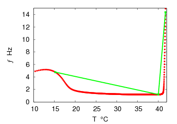 | Figure 3. Frequency f versus temperature T on simulation with the HH model. The frequency passed through a minimum at 38℃and then increased at the higher temperature (Red full circles), on which a certain piecewise line (green line) is put to fit experimental data plots to theoretical curves for the frequency gradient, which will be derived below |
3. Neuron Model and Frequency Gradient Curves
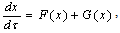
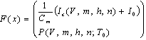
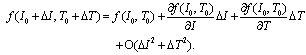
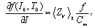
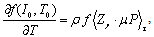
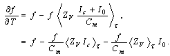
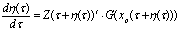
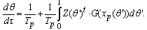
- In Figure 1, we indicate that still-unknown nonlinearities exist in the neuronal firing property. To understand why a firing frequency can be recovered again once it has decreased, and what the mechanism is, the Hodgkin-Huxley (HH) model is employed. The HH model is rewritten with small perturbations of temperature and current, ΔT and ΔI, in the general forms:
 | (1) |
 | (2) |
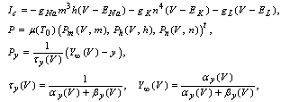 where Cm (= 1 μF/cm2) is the membrane capacity. ENa, EK, and EL are the reversal potentials of Na+, K+ and leak currents respectively, while gNa, gK, and gL are the conductances. μ(T) = (Q10)(T-Te)/10 (Q10 = 3 in this work) rescales time courses of the ion-channel activations with temperature T (◦C) and Te (= 25◦C in this work). αm(V) = -0.1(V + V1) / (exp(-0.1(V + V1)) -1), βm(V) = 4exp(-(V + V2) / 18), αh(V) = 0.07exp(-(V + V3) / 20), βh(V) = 1 / (exp(-0.1(V + V4)) + 1), αn(V) = 0.01(V + V5)/(exp(-0.1(V + V5)) - 1) and βn(V) = 0.125exp(- (V + V6) / 18). We suppose that gNa = 35 mS/cm2, ENa = 55 mV, gK = 9 mS/cm2, EK = -90 mV, gL = 0.1 mS/cm2, EL = -65 mV, V1 = 35, V2 = 60, V3 = 58, V4 = 28, V5 = 34 and V6 = 44 (see[17]) so that the HH model represents an oscillatory system exhibiting repetitive firings via the SNIC bifurcation mechanism (sometimes called the SNIC HH model). It is noticed that the firing frequency gradually decreases and increases again, correspondingly the amplitude of the membrane potential becomes smaller at higher temperature T = 41.6℃. Figure 2 shows the emergence of a small limit cycle (LC) attractor via the SNIC bifurcation around I = 0.161. The LC size varies with an increase in temperature. The bi-stability of the stable equilibrium and the stable LC attractor exists at T = 10℃ (Analysis on the SNIC bifurcation, referred to in Appendix A). In the frequency-current (f-I) curve for T = 10℃, the HH model shows class II excitable, at the same time, class I spiking behaviour. Here the class II means the emergence of oscillation with a nonzero frequency while the class I is a system that begins oscillations with 0-frequency[24],[25]. The SNIC also shows a system that is simultaneously class I excitable and class I spiking at T = 25℃. The SNIC at T = 41.6℃ shows again a system that simultaneously class II excitable and class I spiking. As the results of the f-I curve, we can depict the frequency-temperature (f-T) curve as shown in Figure 3, at I = 0.161. In an increase of T, the frequency decreases to the minimum at 38 ◦C through its peak at 13℃. Immediately afterwards, the frequency slope becomes extraordinary sharp. The f-T curve plays a crucial role in fitting to the V-shaped f-T plot recorded from the hippocampal CA3 pyramid cells. The detailed best-fitting method will be mentioned in the next section.In this work, we select the perturbation G(x) as
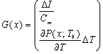 | (3) |
 | (4) |
 | (5) |
 | (6) |
 | (7) |
 | (8) |
 | (9) |
 | (10) |
 Let experimental (f, I, T) data be applied into the H-function. ΔT is the temperature difference between two of 25, 30 and 35℃, namely, ΔT = ± (30 - 25), ± (35 - 30) and ± (35 - 25). ΔI is ±50 pA, which represents the difference of one sampling current to its nearest neighbours.
4. Numerical Calculations
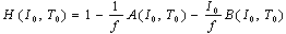
- Next, we calculate the H-function for experimental data on (f, I, T) (called the empirical plot). The H-function is also given by the simulation data of (f, I, T) with the HH neuron (called the theoretical curve). We here investigate how such theoretical curves can fit to the empirical plots. Under the most appropriate condition for the best fitting, the temperature coefficient in the physiological experiment is predicted by rescaling the model temperature in the HH model to the empirical temperature.For the empirical plot, the H(I) is calculated for ΔT = ± (30 - 25), ± (35 - 30) and ± (35 - 25). Figures 4(a) and 4(b) represent respectively the H plots for ΔT > 0 and ΔT < 0 as the functions of I. In analogy, we obtain theoretical curves on simulations with the HH neuron model (solid lines in Figure 4). For this, Ti (i = 0, 1, 2) is sampled on the f-T curve at each current. T0 and T2 are relatively high temperatures while T1 is close to the minimum (see Figure 3). We then select the most appropriate value of Ti (T0 = 15, T1 = 40 and T2 = 41.7) that the theoretical curve passes through the respective plot distribution.In order to confirm that the empirical plot best-fits to the corresponding theoretical curve, we compute confidence that the theoretical curve can be shared with the empirical plot distribution, under an assumption to obey the normal distribution. This confidence is computed as referred to Appendix C. The standard error of the mean is calculated as H1 ± 1.96σ /√n where σ is the standard deviation of the sampling distribution and n = 6. In Figure 5, almost all samplings in plot distribution are of confidence as the corresponding theoretical curve.Finally, we will give additional supporting information to the best fitting by rescaling the temperature coefficient Q10 in the HH neuron. For this, we rescale the temperature coefficient Q10 = 3 in the HH neuron to be in the empirical range of 1.22 ± 0.38 that is calculated in Figure 1(c). In Figures 4 and 5, the temperature ranges for obtaining empirical plots are respectively 5℃ and 10℃. The temperature ranges for obtaining theoretical curves are correspondingly 25℃ and 26.7℃. The rescaled temperature coefficient is thus calculated in the range of 1.24 to 1.51. The range value presumably is satisfied with Q10 = 1.22 ± 0.38 in the experiment.
 | Figure 4. H-I plots for experimental data and its curves for the HH model. (a) ΔT > 0. (b) ΔT < 0 |
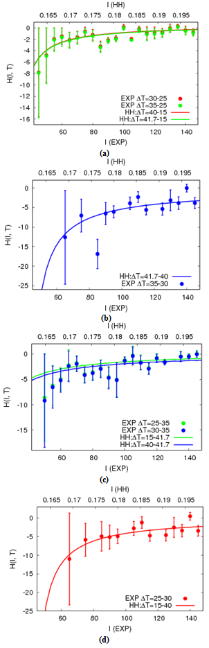 | Figure 5. Theoretical curves best-fit the empirical plots. (a) and (b) are ΔT > 0. (c) and (d) are ΔT < 0 |
5. Discussion and Conclusions
- In this work, we have shown that V-shaped frequency -current responses, recorded from the hippocampal CA3 pyramidal cells, are analytically consistent with the ones simulated with the HH model. However, we cannot declare that the pyramidal cell of the hippocampal CA3 behaves like activations of cold-receptor-like neurons. Rather, in order to ascertain this, we have to examine more in vitro frequency versus current relationships with fine temperature variations of 1-2◦C and then observe the frequency -temperature curve as shown in Figure 3. Also, we have to give physiological reasons of why the frequency increases at 30 - 35 ◦C. Such a frequency increase may result from activations of transient receptor potential (TRP) family of channels such as TRPV3[26-28] and TRPV4[14], which seem to be widely distributed in a brain, are sensitive to body temperature. Both the TRP channels have the temperature threshold of 30 - 35 ◦C for activation, and particularly the TRPV4 channels exist even in the neuronal circuit in the hippocampus.In the theoretical aspects, we have to figure out detailed transition mechanisms of low to high frequencies at T = 41 ◦C. To figure out such transition mechanisms, we analyze the difference of the f-I curves at high and low temperatures. The two dimensional reduced Hindmarsh-Rose model (2DHR)[29] is suitable for clarifying the detailed transition mechanisms or the difference of the two f-I curve, in terms of (9) and (10). The 2DHR model has less complexity than the HH model and retains the analytic tractability of the FitzHugh- Nagumo model[30]. All bifurcations of the Hopf, the SNIC and the SN are computed with appropriate parameter sets in the 2DHR model. Drawing the whole diagram of these bifurcations, the corresponding[∂f / ∂T]-I curve will also be calculated. We thus expect to find differences of the two f-I curves with the same class if the[∂f / ∂T]-I curves have obvious differences.Figure 1(b) showed a decreased frequency with the temperature increase in individual neurons. However in Figure 1(c), the statistic property of the frequency was the monotonic increase, although it was very slight. This indicates the increased activities of the assemblies, in which the underlying individual cell paradoxically exhibits the frequency descent with the temperature increase. Such a paradoxical mechanism should be clarified. One of considerable solutions may be to confirm whether or not pyramidal cells in the hippocampal CA3 are sensitive to current fluctuations on the f-I relationships, because it is known that f-I responses are significantly influenced by the Gaussian distributed current[31]. In addition, under a statistical assumption of empirical plots obeying the Gaussian distribution, the linearity of the log(f)-T is obtained as shown in Figure 1(c). This implies that the Gaussian distributed current contributes to finding a positive slope of the log(f)-T.In order to confirm the statistical assumption, we should do simulations on the HH models with the current fluctuated by Gaussian distribution, analogous to the work of[31] for investigating effects of the variation on f-I responses. Also, the H-I curve for the HH model obeying the Gaussian distribution will be calculated for finding the most suitable variance for best-fit to the empirical plots. Doing such studies becomes more valuable, in comparison with the other cases such as the Gamma, Poisson and exponential interspike interval distributions. This is because we have to show which distribution is of significant essence for understanding the mechanisms of neural information processing[32].We have to discuss if it is necessary to visualize even spike patterns of pyramidal cells in the hippocampal CA3 slice, because it is shown that the spike patterns of neocortical layer 2/3 and 5/6 pyramidal cells change with temperature. The change in spike pattern is due to temperature-dependent changes in the intrinsic properties of the pyramidal cells[33],[34]. To understand such physiological mechanisms on the spike pattern generations of regular spikes, slow frequency adaptation and bursting, we will have to study and model the complex dynamics of various types of the ion channels, referring to[25],[35]. This gives arise to an additional issue if we understand rigorously the detailed dynamics of the ion channels for the sake of the modeling.To the additional issue, we may answer as follows: spike pattern observed in the recording duration as well as detailed channel structures on the current dynamics is not so important in fitting analysis on the temperature controlled frequency-current curve. In our theory, we assume a stable periodic solution for unperturbed firing dynamics, to derive the phase equation and the frequency gradient equation. The stable periodic solution is regardless of any spike pattern such as regular spiking and bursting. Moreover, we can assume the recording duration of 2 sec in the experiment as the one periodic solution. Such assumptions enable us to obtain the frequency gradient equation corresponding to the experimental data.In conclusion, with respect to the temperature sensitive activities on neurons, the fact that the frequency increases with temperature reduction and paradoxical response when the temperature is increased can be regarded to be of importance for information processing in the brain. We then predict that such temperature sensitive activities are potentially observed even in the hippocampal CA3 pyramidal cells. To support this prediction, we propose an experimental data fitting method of a frequency gradient curve for current and temperature simulated with the SNIC HH oscillator. In this method, the theoretical curves were established by expanding the HH oscillator with small perturbations of I and T while the empirical plot was also obtained with f-I responses recorded from the hippocampal CA3 pyramidal cells at different temperatures. The empirical plot was best fitted to the theoretical curve under a certain temperature range on simulations with the HH oscillator. The next task in the future is to confirm that the experimental data analysis proposed in this work is a useful and powerful method. For this, we will have to study more the experimental data fitting method by using the ML model, the 2DHR model and the bursting model, which undergo the SNIC bifurcation mechanism with or without slow spike frequency adaptation. In addition, we suppose it very interesting to simulate the HH model with Gaussian noise for getting the higher reproducibility of the empirical plot. This is because we can easily expect that theoretical curves computed with the Gaussian distributions cover the empirical data plot when the noise intensity is larger.
ACKNOWLEDGEMENTS
- The authors thank Natsume at Kyushu Institute of Technology and Aihara at The University of Tokyo for fruitful and active discussions. Y.I. was supported by the Funding Program for Next Generation World-Leading Researchers (no. LS023).
Appendix A. Analysis on Stabilities of Stationary Solutions
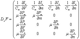
- The stability analysis of the differential equations was briefly reviewed. The detailed analysis is referred to[36],[37]. We analyzed the character of the equilibrium points x0 of[dx/dτ] = 0. This was done by linearizing the HH model without the perturbation term, close to x0 and by solving the characteristic equation
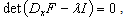 | (A.1) |
 | . (A.2) |
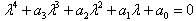 | (A.3) |
Appendix B. Phase Reduction Method
- The detailed derivation is referring to[18],[19]. Supposing a small perturbation in the HH oscillator, the phase reduction method should be applied to:
 | (B.1) |
 | (B.2) |
 | (B.3) |
 | (B.4) |
 | (B.5) |
 | (B.6) |
 | (B.7) |
 | (B.8) |
 | (B.9) |
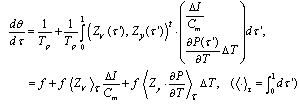
Appendix C. Averaged Frequency gradient equations
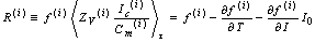
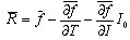
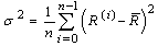
- Let the sampling index be i (= 0, ..., n - 1), that is, the number of pyramid cells employed for recording in the experiment, referring to[23]. The ith neuron’s equation for frequency gradient is
 | (C.1) |
 | (C.2) |
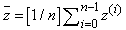 . Then, both the sides are divided over averaged frequency:
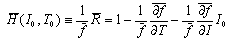 | (C.3) |
 | (C.4) |
References
| [1] | E. Dodt, Y. Zotterman, "The Discharge of Specific Cold Fibres at High Temperatures; the paradoxical cold", Acta Physiol. Scand., vo1.26, no.4, pp.358-65, 1952. |
| [2] | R. R. Long, "Sensitivity of cutaneous cold fibers to noxious heat: paradoxical cold discharge", J. Neurophysiol., vol.40, no.3, pp.489-502, 1977. |
| [3] | H. Hensel, A. Iggo, I. Witt, "A quantitative study of sensitive cutaneous thermoreceptors with C afferent fibres", J. Physiol., vol.153, pp.113-126, 1960. |
| [4] | R. K. Adair, "A model of the detection of warmth and cold by cutaneous sensors through effects on voltage-gated membrane channels", Proc. Natl. Acad. Sci. USA, vol.96, no.21, pp.11825-11829, 1999. |
| [5] | A. L. Hodgkin, A. F. Huxley, "A quantitative description of membrane current and its application to conduction and excitation in nerve", J. Physiol., vol.117, no.4, pp.500-544, 1952. |
| [6] | Y. D. Sato, "Temperature Controlled Voltage Oscillation in Neural Circuit Undergoing Homoclinic Bifurcation", International Journal of Modern Engineering Research, vol.2, no.4, pp. 2728-2734, 2012. |
| [7] | Y. D. Sato, K. Okumura, A. Ichiki, M. Shiino, H. Cateau, "Temperature-modulated synchronization transition in coupled neuronal oscillators", Phys. Rev. E vol.85, 031910-12, 2012. |
| [8] | C. Morris, H. Lecar, "Voltage oscillations in the barnacle giant muscle fiber", Biophys. J., vol.35, no.1, pp.193-213, 1981. |
| [9] | H. Lecar, "Morris-Lecar model", Scholarpedia vol.2, no.10, 1333, 2007. |
| [10] | J. Keener, J. Sneyd, "Mathematical Physiology", Springer- Verlag, New York, 1998. |
| [11] | A. I. Hogkin, B. Katz, "The effect of temperature on the electrical activity of the giant axon of the squid", J. Physiol. (Lond) vo.109, pp.240-249, 1949. |
| [12] | J. M. Ritchie, R. W. Straub, "The effect of coolingon the size of the action potential of mammalian non-medullated fibers", J. Physiol. (Lond) vol.134, pp.712-717, 1956. |
| [13] | E. Moser, I. Mathiesen, P. Andersen, "Association between brain temperature and dentate field potentials in exploring and swimming rats", Science vol.259, pp.1324-1326, 1993. |
| [14] | K. Shibasaki, M. Suzuki, A. Mizuno, M. Tominaga, "Effects of Body Temperature on Neural Activity in the Hippocampus: Regulation of Resting Membrane Potentials by Transient Receptor Potential Vanilloid 4", J. Neurosci., vol.27, no.7, pp. 1566-1575, 2007. |
| [15] | M. Mizunuma, N. Takahashi, A. Usami, N. Matsuki, Y. Ikegaya, "High temperature, but not high pressure, conditions alter neuronal activity", J. Pharmacol. Sci., vol.110, pp.117-121, 2009. |
| [16] | C.-B. Lu, Z.-H. Wang, Y.-H. Zhou, M. Vreugdenhil, "Temperature- and concentration-dependence of kainate-induced γ oscillation in rat hippocampal slices under submerged condition", Acta Pharmacol. Sin., vol.33, no.2, pp.214-220, 2012. |
| [17] | X.-J. Wang, G. Buzsaki, "Gamma Oscillation by Synaptic Inhibition in a Hippocampal Interneuronal Network Model", J. Neurosci. vol.16, no.20, pp.6402-6413, 1996. |
| [18] | F. C. Hoppensteadt, E. M. Izhikevich, "Weakly Connected Neural Networks", Springer, New York, 1997. |
| [19] | A. Mehrotra, A. Sangiovanni-Vincentelli, "Noise Analysis of Radio Frequency Circuits", Kluwer, Dordrecht, 2004. |
| [20] | Y. D. Sato, "Synchronization Phenomena in a Pair of Coupled Neuronal Oscillator Systems", Doctoral Dissertation, Tokyo Institute of Technology, Japan, 2005. |
| [21] | T. Sasaki, N. Matsuki, Y. Ikegaya, "Action-potential modulation during axonal conduction", Science, vol.331, no.6017, pp.599-601, 2011. |
| [22] | N. Takahashi, K. Kitamura, N. Matsuo, M. Mayford, M. Kano, N. Matsuki, Y. Ikegaya, "Locally synchronized synaptic inputs", Science, vol.335, no.6066, pp.353-356, 2012. |
| [23] | J. H. Zar, "Biostatistical analysis 4th edition", Prentice-Hall, Inc. Upper Saddle River, New Jersey, 1999. |
| [24] | E. M. Izhikevich, "Neural Excitability, Spiking, and Bursting", International Journal of Bifurcation and Chaos, vol.10, no.6, pp. 1171-1266, 2000. |
| [25] | E. M. Izhikevich, "Dynamical Systems in Neuroscience: The Geometry of Excitability and Bursting", MIT Press, Cambridge, MA, 2007. |
| [26] | A. M. Peier, A. J. Reeve, D. A. Andersson, A. Moqrich, T. J. Earley, A. C. Hergarden, G. M. Story, S. Colley, J. B. Hogenesch, P .McIntyre, S. Bevan, A. Patapoutian, "A heat-sensitive TRP channel expressed in keratinocytes", Science, vol.296, no.5575, pp.2046-2049, 2002. |
| [27] | H. Xu, I. S. Ramsey, S. A. Kotecha, M. M. Moran, J. A. Chong, D. Lawson, P. Ge, J. Lilly, I. Silos-Santiago, Y. Xie, P. S. DiStefano, R. Curtis, D. E. Clapham, "TRPV3 is a calcium-permeable temperature-sensitive cation channel", Nature, vol.418, no.6894, pp.181-186, 2002. |
| [28] | G. D. Smith, M. J. Gunthorpe, R. E. Kelsell, P. D. Hayes, P. Reilly, P. Facer, J. E. Wright, J. C. Jerman, J. P. Walhin, L. Ooi, J. Egerton, K. J. Charles, D. Smart, A. D. Randall, P. Anand, J. B. Davis, "TRPV3 is a temperature-sensitive vanilloid receptor-like protein", Nature, vol.418, no.6894, pp. 186-190, 2002. |
| [29] | S. Tsuji, T. Ueta, H. Kawakami, H. Fujii, K. Aihara, "Bifurcations in Two-dimensional Hindmarsh-Rose Type Model", Int. J. Bifurcat. Chaos, vol.17, no.3, pp.985-998, 2007. |
| [30] | R. FitzHugh, "Mathematical models of excitation and propagation in nerve", Chapter 1 pp. 1-85 in H. P. Schwan, ed. Biological Engineering, McGraw-Hill Book Co., N. Y., 1969. |
| [31] | M. Arsiero, H.-R. Luscher, B. N. Lundstrom, M. Giugliano, "The Impact of Input Fluctuations on the Frequency-Current Relationships of Layer 5 Pyramidal Neurons in the Rat Medial Prefrontal Cortex", J. Neurosci., vol.27, no.12, pp.3274- 3284, 2007. |
| [32] | H. Cateau, A. D. Reyes, "Relation between single neuron and population spiking statistics and effects on network activity", Phys. Rev. Lett., vol.96, 058101-4, 2006. |
| [33] | J. Waters, F. Helmchen, "Background Synaptic Activity Is Sparse in Neocortex", J. Neurosci. vol.26, no.32, pp.8267- 8277, 2006. |
| [34] | T. Hedrick, J. Waters, "Effect of temperature on spiking patterns of neocortical layer 2/3 and layer 6 pyramidal neurons", Front. Neural Circ., vol.6, 28-10, 2012. |
| [35] | T. Aoyagi, N. Terada, Y. Kang, T. Kaneko, T. Fukai, "A bursting mechanism of chattering neurons based on Ca2+- dependent cationic currents", Neurocomputing, vol.38-40, pp. 93-98, 2001. |
| [36] | P. Arhem, G. Klement, C. Blomberg, "Channel Density Regulation of Firing Patterns in a Cortical Neuron Model", Biophys. J., vol.90, pp.4392-4404, 2006. |
| [37] | H. Zeberg, C. Blomberg, P. Arhem, "Ion Channel Density Regulates Switches between Regular and Fast Spiking in Soma but Not in Axons", PLoS Comp. Biol., vol.6, no.4, e1000753, 2010. |