1. Introduction

The northern Indian Ocean is usually subdivided into two different subregions according to differences in surface water properties [16,12], the Arabian Sea having high salinity water and the Bay of Bengal low salinity water. The salinity increases from the west to the east and from the equator towards the north. The east part of the Indian Ocean is mostly affected by the rainfall region around Sumatra which contributes to the sea surface low salinity observed in the Bay of Bengal [6,15].

In general terms, the surface circulation in the Indian Ocean follows the wind pattern. For example, [18], organizes the Indian Ocean into three general circulation systems: the seasonal monsoon gyre, the subtropical anticyclonic gyre of the Southern Hemisphere and the Antarctic waters with the circumpolar current. In fact, it is seasonal reversal of the monsoonal gyre that gives the Indian Ocean its principal and unique characteristics. Figure 1 shows the main features of the Indian Ocean circulation.

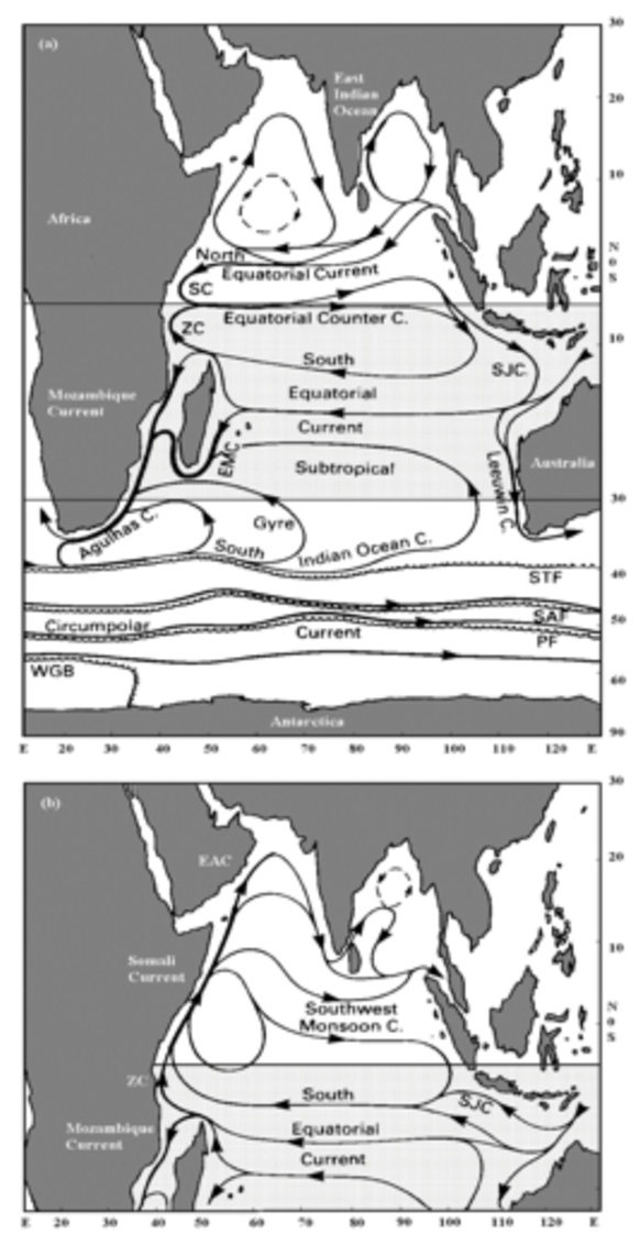Figure 1. Surface currents in the Indian Ocean. (a) NE Monsoon (Dec-April); (b) SW Monsoon (Jun-Oct). EAC = East Arabian Coast; SJC = South Java Current; ZC = Zanzibar Current; EMC = East Madagascar Current; SC = Somali Currents; STF = Subtropical Front; SAF = Sub-Antarctic Front; PF = Antarctic Polar Front; WGB = Weddell Gyre Boundary. Adapted from [14]

During the NE Monsoon, a thermohaline circulation with northward transport against the wind direction occurs along the west coast of India. This northward current is generated by differences in pressure gradient from north to south caused by differences in temperature and salinity during the winter [14]. A remarkable semi-annual event which occurs in the study area is the Equatorial Jet, first described by [16]. It is a strong eastward jet flow that occurs during the transition between the monsoons [16,9,10]. The Equatorial Jet that flows between 2° N and 2° S results in the deepening of the thermocline along the Sumatran coast and uplift of the thermocline along the African coast [9,5]. It represents a semi-annual reversal of flow triggered mainly by the zonal wind, although it is not the only mechanism responsible for the event as it is also influenced by equatorial Kelvin waves at greater depths. The situation is reversed when wind decreases speed and a westward flow, together with the South Equatorial Current, replaces the water off Africa [14,5].

The salinity is below or close to 34 for most of the year in the eastern part of the Indian Ocean, along 10° S. This low salinity is due to the proximity of the AAMW which enters the Indian Ocean between the Indonesian islands and north of Australia. Another interesting aspect related to the Indian Ocean circulation is the weak eastern boundary current along the Australian coast compared to a strong western boundary current along the African coast (Agulhas Current) [2,7,3].

This work describes the salinity distribution in the surface layer of the tropical Indian Ocean (25° N to 30° S and 30° E to 120° E) based on analysis of semi-annual and annual amplitudes of temperature and a multiple regression analysis between temperature, Ekman pumping, components of pseudo-stress wind, wind magnitude and net-down-freshwater-flux.

2. Material and Methods

A set of 5° grid average sea surface temperature (SSTS) contour plots for the Indian Ocean is produced based on the NODC_WOA94 data provided by the NOAA/OAR/ESRL PSL. Salinity, together with the independent variables wind, ndff (net-down-fresh-water-flow) and Ekman pumping, are included in a multiple regression analysis to define the relative importance of each one of these variables in the physical processes at the surface of the Indian Ocean. The ndff data set is based on COADS (Comprehensive Ocean-Atmosphere Data Set) and obtained from [8]. It is originally organized in a 2×2 grid and averaged in 5×5 grid for this research. The ndff represents the balance between precipitation and evaporation (P-E) and its unit is mm. The wind data is obtained from the Florida State University (FSU) Wind Stress Data Set for the tropical Indian Ocean in a 1×1 grid. The data is averaged in a 5×5 grid. The FSU data set is based on COADS and NCDC (National Climatic Data Centre). The wind stress is presented as pseudo-stress wind, which is the wind component times the wind magnitude. For salinity, the twelve-monthly mean values are subjected to a Harmonic Analysis to determine two harmonic components, one having a period of one year and the other a period of six months. The process aims to examine how the two components contribute and interact to produce the more complex cycle of the observed and modelled data.

The harmonic terms are considered to be stationary, as the averages and corresponding autocorrelations are not expected to vary significantly in a long period of time. In this way, the stationary time series of salinity can then be expressed symbolically by Fourier series as a cosine function in which the first and second harmonic terms are multiplied by the maximum amplitude of the variable and added to the mean annual parameter. The modelled data can thus be expressed as:

where:

O(t) = observed value as a function of time where t is time in days, since the start of an arbitrary year,

= mean value over the period analysed,

A = Amplitude of the annual harmonic component,

B = Amplitude of the semi-annual harmonic component,

a = Phase-lag of the annual component,

b = Phase-lag of the semi-annual component,

ω_a = Angular frequency which represents the increment in phase per unit time, t, of the annual harmonic component,

ω_s = ditto for the semi-annual component but

= phase of the annual harmonic,

= phase of the semi-annual harmonic.

Values of O, A, B, a and b are to be determined by analysis. They represent the average annual salinity and is a positive constant. The amplitude value (A or B) is also a positive constant that represents the amplitude of the motion and so its maximum departure from the mean value as the term oscillates within a range of + or -. Phase-lag is expressed in degrees and increments at 30° per month for the first harmonic and 60° per month for the second, where phase is zero it implies that a maximum occurs in the beginning-January. It expresses the average time when the maximum of SSS occurs within the annual cycle. For example, phase of 120° corresponds to first of April, 150° first of May and 270° first of October. The sum of square residual is defined as:

and represents the sum of squared differences between observed (Y) and the predicted values (Y’), these differences representing the small inadequacies of the fit.

3. Results

The 5° grid average sea surface temperature (SSS) contour plots during the SW Monsoon (July, August, and September) can be seen in Figure 2. The salinity contours tend to be zonally orientated away from the coast, while a meridional influence is observed close to the boundaries. A typical zonal pattern of salinity distribution is observed only south of 10° S. The salinity contours follow a more meridional pattern of distribution elsewhere.

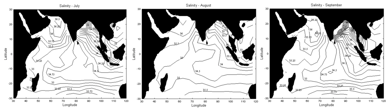Figure 2. Sea surface salinity (psu) contours for the SW Monsoon (July, August, and September). Data Source: NODC_WOA94 data provided by the NOAA/OAR/ESRL PSL

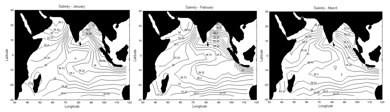Figure 3. Sea surface salinity (psu) contours for the NE Monsoon during the months of January, February and March. Data Source: NODC_WOA94 data provided by the NOAA/OAR/ESRL PSL

The annual variation of salinity, as expressed through the amplitude of the annual (first) and semi-annual (second) harmonic, can be seen in Figure 4. Annual amplitude values higher than 0.20 are observed in the north of the Arabian Sea and the Bay of Bengal, along the southwest coast of India in the Arabian Sea, and towards the north along the western and eastern coastlines of the Bay of Bengal (Figure 4a). However, for most of the central Indian Ocean, the annual amplitude of salinity is close to or lower than 0.20.

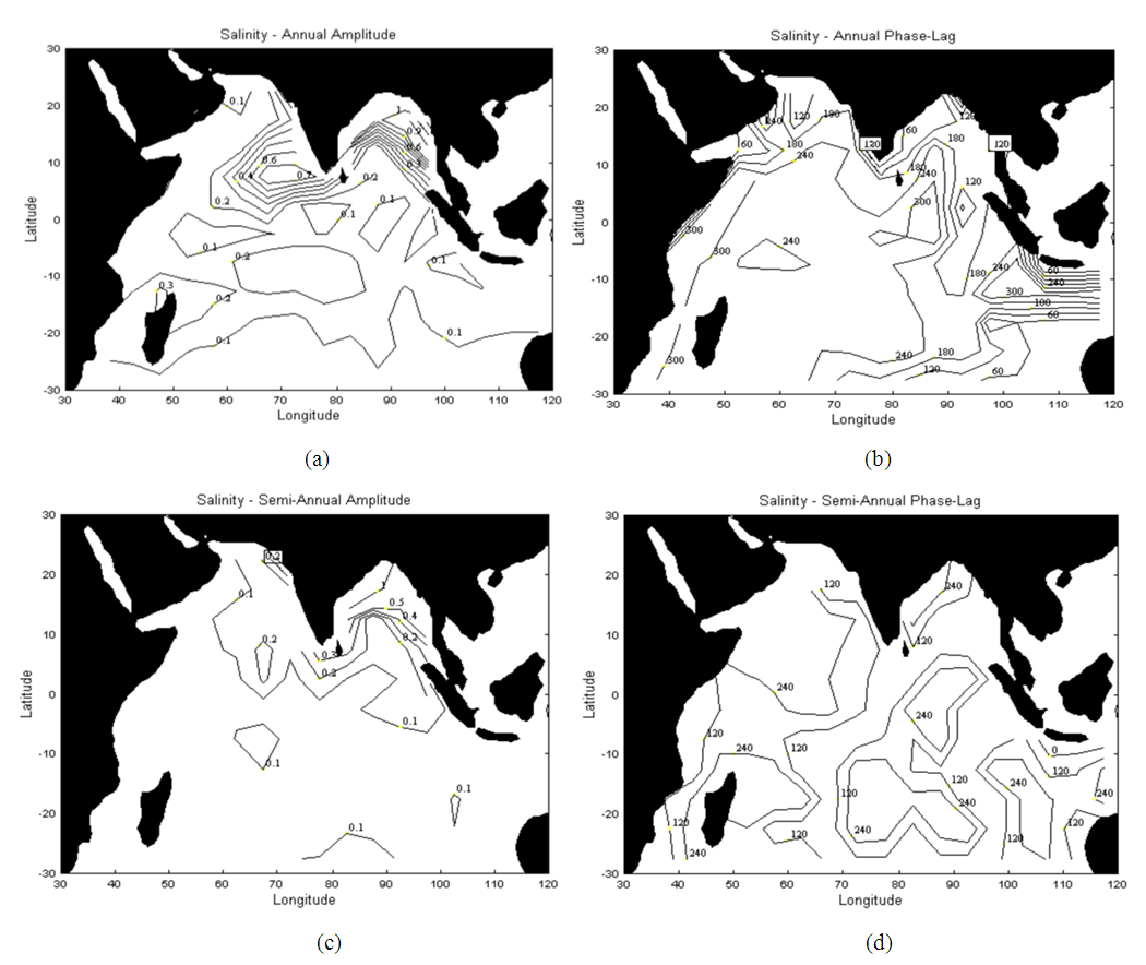Figure 4. (a) The distribution of the SSS amplitude for the first harmonic. (b) The distribution of the phase-lag of salinity for the first harmonic. ( c) The distribution of the SSS amplitude for the second harmonic. (d) The distribution of the phase-lag of salinity for the second harmonic. Amplitude and phase of temperature are calculated from the NODC_WOA94 data provided by the NOAA/OAR/ESRL PSL

Figure 5a exhibits the plots of the observed SSS with the two-component harmonic fit to the observation, the two individual harmonic components and their interaction through the year (5b), and the residual error between observed and harmonic fit, at 72.5º E and 7.5º N (5c) along the Southwest coast of India where large amplitude of salinity values are found. The annual component exhibits a maximum in August and a minimum in February. By comparison, the amplitude of the semi-annual component is smaller in magnitude than that of the annual component, with two maxima in April and October and two minima in July and January (Figure 5b). Phase-lags are only shown for regions where amplitudes are more than 0.20 (northern Indian Ocean). Residual errors between observed and harmonic salinity are below 0.09 for most of the data. Large residuals are observed from September to November, with a maximum of 0.44 in October (Figure 5c). Otherwise, the small magnitude of the residual errors is an indication that salinity variability through the year can be reasonably explained by just the two harmonic components.

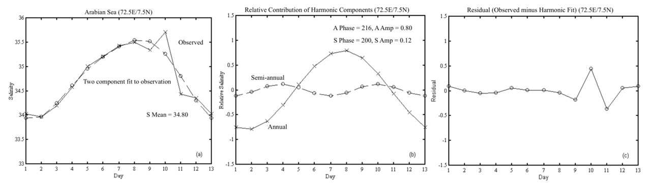Figure 5. (a) Observed and two components fit to observations (psu). (b) First and second components of the harmonic analysis. (c) Residual plot between observed and harmonic salinity (psu). Time (months) in which 13 is equal to 1 and corresponds to mid-January

The distribution of the salinity phase-lag for the annual harmonic component can be observed in Figure 5b. In the Arabian Sea, maximum annual amplitude of salinity is found at the end of August, along the southwest coast of India. The central Bay of Bengal exhibits maximum annual amplitude at late August. In the southern Indian Ocean, the maximum of the annual component occurs at the end of September at 10° S and in late July when close to 30° S.

Large amplitude values related to the western Bay of Bengal can be analysed in Figure 6 which shows the plots of the observed SSS with the two-component harmonic fit (Figure 6a), the two individual relative contributions of the harmonic components (Figure 6b) and the residual error between observed and harmonic fit (Figure 6c), at 82.5º E and 17.5º N.

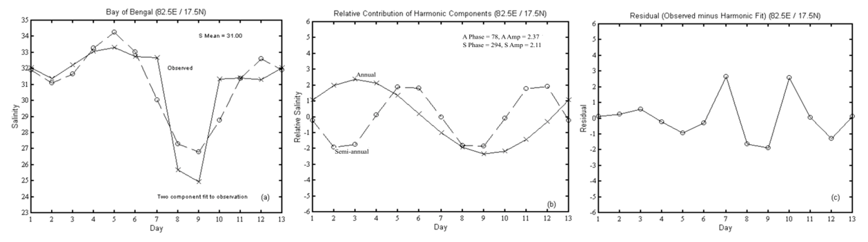Figure 6. (a) Observed and two components fit to observations (psu). (b) First and second components of the harmonic analysis. (c) Residual plot between observed and harmonic salinity (psu). Time (months) in which 13 is equal to 1 and corresponds to mid-January

Two salinity maxima are observed during May and December and two minima during February and August (Figure 6a). The amplitudes for the annual and semi-annual harmonic terms are similar in magnitude (Figure 6b). The annual component is seen to have a maximum in March (peak of the NE Monsoon) and a minimum in August (peak of the SW Monsoon) which suggests a connection with the monsoons. For the semi-annual harmonic term, two maxima are seen during May/June and October/November and two minima during February/March and July/August. The two minima are associated with the transition between the monsoons, and the two maxima are related to the peak of the monsoons.

The distribution of the harmonic terms (Figure 6b) demonstrates how the two harmonic components combine. It can be seen from this Figure that the annual and semi-annual harmonics from January to April are in opposition and produce a minor low trough of salinity during February. The two harmonic components act in conjunction during August and September which results in a pronounced minimum observed during this period.

Multiple regression analysis is performed for the whole study area and the final regression equations with an adjusted R² larger than 0.6 are shown in Table 1. Components of wind stress, wind magnitude, Ekman pumping and ndff are affecting the dependent variables, but the Wx is a constant presence for all equations, except for the location at 72.5° E and 7.5° N. In addition, Wx and Wy exhibit larger values for Beta coefficients which indicates its importance, among the variables, for the variability of the dependent variables (Table 2).

Table 1. Predicted equations for the western Arabian Sea. Wx = zonal component of pseudo-stress wind (m2s-2), Wy = meridional component of pseudo-stress wind (m2s-2), ndff = net-down-fresh-water-flux (mm), Ekman pumping = (-) downward/(+) upward (x10-3 kg.m2.s-1), S = salinity (psu), Wmg = wind magnitude (ms-1)

The correspondent residuals of the multiple regression analysis at 57.5 E/17.5 N are shown in Figure 7. The adjusted R², the standard error and the final regression equation for salinity is indicated in the graph. To assess the relative importance of the independent’s variables presented in the regression equations (Table 2), the Beta coefficients can be used and are exhibited in Table 2.

A better fit can be seen between observed and predicted salinity, with an adjusted R² of 0.89. The low residual errors observed in Figure 7 show that salinity can be well explained by the Wx, Wy, Wmg and ndff (Table 2). The meridional component of the wind stress represents the most important variable to the salinity variability (Wy=7.2), followed by Wx, Wmg and ndff.

Table 2. Beta coefficients between dependent and independent variables at 57.5° E and 17.5° N. Wx = zonal component of pseudo-stress wind, Wy = meridional component of pseudo-stress wind, ndff = net-down-fresh-water-flux and Wmg = wind magnitude

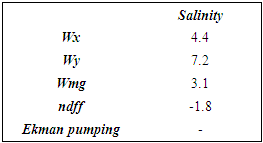
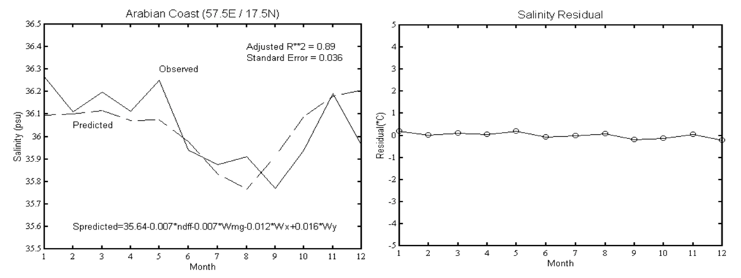Figure 7. Comparison between observed and predicted salinity from multiple regression equation at 57.5°E and 17.5°N

4. Discussion

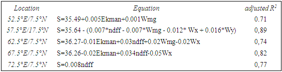
The highest salinity found in the north of the Arabian Sea, increasing from the equator and southward, while the lowest salinity values are observed in the Bay of Bengal, agrees with the influence of the ndff in the eastern equatorial zone and in the Bay of Bengal. For example, a maximum positive ndff of 160 mm.yr^-1 is observed at the equator at about 95° E and 5° S, which coincides with a low salinity of about 34.10. On the other hand, the two evaporative basins observed in the western Indian Ocean and south of the equator coincides with salinity values above 35.00.

The low salinity tongue with salinities below 35.00, observed along 10°S, is a result of the westward transport of the low salinity waters from the Australasian Mediterranean Sea [15]. To the north of the Bay of Bengal the annual amplitude can be close to 2.00, influenced by the river runoff from the Ganga and Brahmaputra rivers and by the advection of low salinity water from Bay of Bengal. However, for most of the central Indian Ocean, the annual amplitude of salinity is close to or lower than 0.20. As a comparison, a similar situation is observed in the North Sea where higher amplitudes are found close to the inflow of the rivers Rhine and Elbe and lower amplitudes are observed in the open sea [4,1].

In the northern Indian Ocean, the latest occurrence of the maximum of the annual component, end of August, is found in the southeast part of the Arabian Sea and in the Bay of Bengal. In the central Arabian Sea, the annual component exhibits its maximum from late April to early July. The variability of the maximum of the annual components observed in the Indian Ocean is consistent with the distribution of the ndff contours. During the SW Monsoon, the ndff becomes gradually positive towards the east, in the direction of the west coast of India, which results in a peak of maximum salinity in August and decreasing afterwards. During the NE Monsoon, the ndff is negative elsewhere in the Arabian Sea.

The strong meridional gradient in the distribution of the maximum of the annual components, observed in the central part of the Bay of Bengal from early May to early September, can be related to the lowest salinity that occurs in August, which coincides with a maximum ndff. In the central Bay of Bengal, the maximum of the annual component that occurs at early September and early May in the east of the region, can also be a result of the ndff distribution which is larger along the eastern boundaries of the Bay of Bengal.

The maximum annual component, observed in August and a minimum in February, shows a connection with the summer and winter. During August, the peak of the SW Monsoon, the maximum of the annual component is associated with a maximum salinity. Since this is considered the wet season in which high precipitation is observed in India, low salinity values should be expected. This can be explained by the influence of the East Arabian Current, which advects high salinity waters from west to east in the Arabian Sea. During February, the peak of the NE Monsoon, the circulation reverses and a westward flow dominates the Arabian Sea. The low salinity associated with the minimum of the annual component can be a result of the influence from the early East Indian Winter Jet (EIWJ). The EIWJ, fully established by November, supplies fresh and low-density water from the Bay of Bengal into the Arabian Sea, which could explain the low salinities values observed in the area.

The two minima of the semi-annual component, observed in July and January, are related to the beginning of the SW Monsoon and NE Monsoon while the two maxima occur later in the monsoons, close to the transition months between the monsoons. It is clearly seen that the annual term plays a dominant role in determining the maximum and minimum salinity observed during August and January, while the semi-annual component provides minor adjustment.

The annual component shows the influence of the monsoons through the year, with a high salinity during the NE Monsoon and a secondary peak of salinity during the SW Monsoon. From mid-February to mid-April, the first maximum of the annual component seems to be mainly a result of the wind-driven monsoon. During this time, the anticyclonic flow (EIC) in the Bay of Bengal brings higher salinity waters from the equator and along the eastern Indian coast. The second maximum of the annual component, from mid-July to mid-September, is related with the effects of the East Arabian Current, which brings high salinity waters from the Arabian Sea along the western Indian coast. This influence is seen by the increase in salinity from August to November.

The two salinity highs are associated with the two maxima of the semi-annual components, and the two salinity lows are associated with the two minima. The two minima are related with the peak of the NE and SW Monsoon. During the NE Monsoon it acts in opposition with the annual cycle and can be related with the local weak anticyclonic flow. During the SW Monsoon the low salinity during July and August can be related to the increase in precipitation which is then suppressed by the influence of the high salinity waters from the Arabian Sea.

The two maxima occur during the transition of the monsoons when the winds are weaker, but the area is likely to be influenced by the higher salinity waters advected by the East Arabian Current from the Arabian Sea. On the one hand, in November, the anticyclonic flow is replaced by the East Indian Winter Jet, which brings low salinity waters from the equator into the Bay of Bengal. On the other hand, from May, large precipitation and river runoff decrease the salinity at the sea surface. However, care must be taken when analysing the salinity variability during the SW Monsoon, as large residual errors are observed during this period.

In consequence, it is suggested that the minimum and maximum salinities can be a result of different processes such as precipitation and wind direction. For example, the direction of the zonal component of the wind stress is westward during January and February and eastward during August. Therefore, the minima during winter could reflect the influence of freshwater advected from the Indonesian archipelago. This secondary low is likely to be associated with the direction of the components of the wind stress (eastward and southward) as a negative ndff is observed during this season. This is an indication that advection processes can be important, affecting the decrease in salinity during this period.

The minimum during summer could be, at least in part, a result of the high precipitation along the eastern boundaries of the Bay of Bengal during this season. During the SW Monsoon, the winds carry moist air from the central Arabian Sea towards India, where it precipitates. Therefore, high precipitation associated with river runoff results in strong salinity gradients in the Bay of Bengal, especially along the coast where freshwater input is larger. The maximum observed during May and November, at the time of the transition of the monsoons, can be associated with the decrease in wind-induced evaporation combined with advection processes.

The importance of the Wy and Wx variables in the regression equation can be associated with the advection processes that take part in the western Arabian Sea region. During summer (SW Monsoon) the area is dominated by the East Arabian Current that advects high salinity from west to east. This flow reverses during winter (NE Monsoon) and low salinity waters are advected westward. The increase in salinity from February to June, in the eastern Arabian Sea, follow the increase in Wx and Wmg. Ekman pumping exhibits a dramatic increase in downwelling from May to July, and then an abrupt increase from July to November. The minimum of Ekman pumping from June to August coincides with the maximum of the pseudostress wind components and wind magnitude.

5. Conclusions

Large annual and semiannual amplitudes of salinity were identified in the Bay of Bengal and along the western Indian coast. Salinity could only be explained by the independent variables in few locations. This is probably due to advection processes that take part in the role of salinity variability. For example, the reversal of the zonal circulation in the Arabian Sea from one monsoon to the other. This reversal transports water of high salinity from the west to the east during the SW Monsoon, and to the opposite direction during the NE Monsoon, results in a strong meridional gradient of salinity in the central Arabian Sea. In the north of the Bay of Bengal, the influence of river runoff also seems to play a major role in the variability of the sea surface salinity, especially in the coastal areas. The difficulty in predicting salinity, especially along the western Arabian Sea can be explained by the advection of low salinity water masses from the Southern Hemisphere, during the SW Monsoon. This influence is not considered in the correlation analysis. Besides the advection influence, coastal upwelling is also lacking in the multiple regression analysis. As it is not treated as an independent variable, the approach adopted is the relation between the wind components and the orientation of the coastline. As can be seen from the multiple regression analysis, this approach is not very satisfactory along the western Arabian Sea, where the coastal upwelling is important. Although salinity could not be explained by the variables, the analysis of the variability of the individual variables, such as ndff and components of the pseudostress wind, associated with the results of harmonic analysis, could provide a reasonable picture of the processes related to the salinity variability. Nevertheless, salinity tends to exhibit a uniform pattern of distribution over the ocean's surface, except for the Bay of Bengal region and eastern equatorial region.

ACKNOWLEDGEMENTS

This study was supported by the Flinders University of South Australia. Special thanks to Matthias Tomczak, always a source of inspiration and support.