-
Paper Information
- Paper Submission
-
Journal Information
- About This Journal
- Editorial Board
- Current Issue
- Archive
- Author Guidelines
- Contact Us
Marine Science
p-ISSN: 2163-2421 e-ISSN: 2163-243X
2014; 4(3): 59-63
doi:10.5923/j.ms.20140403.01
On the Kolmogorov Spectra in the Field of Nonlinear Wind Waves
 Abstract
 Reference
 Full-Text PDF
 Full-text HTML
1A. M. Obukhov Institute of Atmospheric Physics of RAS, Moscow, 119017, Russia
2School of Advanced sciences, VIT University, Chennai, 600127, India
Correspondence to: Vlad Polnikov, A. M. Obukhov Institute of Atmospheric Physics of RAS, Moscow, 119017, Russia.
| Email: |  |
Copyright © 2014 Scientific & Academic Publishing. All Rights Reserved.
The nature of Kolmogorov spectra formation in the field of nonlinear wind waves are discussed. The currently dominating assertion is that such spectra for wind waves are formed as stationary solutions of the kinetic equation, which describes the conservative nonlinear four-waves resonant interactions. However, this statement here is is refuted by direct numerical calculations of the kinetic integral. Using two independent methods of calculating the kinetic integral for nonlinear surface waves in deep water, it is shown that the theoretical spectra of Kolmogorov type, found by Zakharov and co-authors [4, 7], are not stationary on a limited frequency band. Conditions for the existence of Kolmogorov spectra in real wind waves and possible mechanisms of their formation are discussed.
Keywords: Kolmogorov spectra, Kinetic integral, Numerical calculations, Wave energy flux, Wave action flux
Cite this paper: Vlad Polnikov, G. Uma, On the Kolmogorov Spectra in the Field of Nonlinear Wind Waves, Marine Science, Vol. 4 No. 3, 2014, pp. 59-63. doi: 10.5923/j.ms.20140403.01.
Article Outline
1. Introduction
- More than 70 years ago, Kolmogorov [1] has expressed the hypothesis that in a random, statistically homogeneous and stationary velocity field of the turbulent flow, some stable statistical forms can exist (structural functions), which are determined only by the flow of certain physical quantity (for example, the kinetic energy dissipation rate, ε, having dimension L2T-3). In the following paper, Obukhov [2] has applied this hypothesis for derivation of the spatial spectrum of turbulent speed field. He has found the spectrum of the form,
 , in which the dimensional constant, с, is proportional to ε2/3. Thus, the spectrum is really defined by the only constant, ε, which has also the meaning of the flux of kinetic energy through the wave number scale, k. Such spectra are called as Kolmogorov–Obukhov spectra, herein referred to as the Kolmogorov spectra [3]. There are a lot of observations of Kolmogorov’s type spectra in real natural processes [3]. 25 years later, Zakharov and Filonenko [4] have showed analytically that in the case of infinite axes of wave numbers k, the Kolmogorov’s type spectra can exist as an exact stationary solution of the four-wave kinetic equation (KE). For the random field of nonlinear surface waves in water, KE can be written in the form1
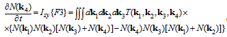 | (1) |
 | (2) |
 | (3) |
 and they are isotropic in angle
  . In [4] it was found that the solution
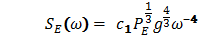 | (4) |
 | (5) |
 | (6) |
2. Computational Details
- To address the first part of the task, two independent kinetic integral calculation algorithms are used, described in [12], [13]. As the integrand, the special (academic) spectra of the following frequency-angular presentation are used
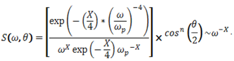 | (7) |
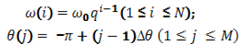 | (8) |
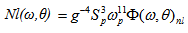
 . In this case, the peak frequency is ωp = 1, and the upper-edge frequency is ωm = ω(61) = 10.4, that provides a sufficiently large frequency range, where the stable calculated values of nonlinear transfer are realized, not depending on the choice of ωo and ωm.It should be noted here that earlier in [12], the basic properties of kinetic integral were studied by the authors for the fast falling spectra (X> 4), when the kinetic integral is well defined. This allowed us to restrict ourselves by sufficiently small values of ωm/ωp not exceeding 4. But for weakly decaying spectra of forms (4) and (5), the convergence of Ist is severely weakened (since the kernel T of Ist is depending on the frequency alike ω12 [12]), which is manifested by a dependence of the nonlinear transfer at frequency ω on the magnitude of ωm, especially in the vicinity of ωm (so called “the edge effect” of a limited bandwidth). However, for large values of ωm, the amount of nonlinear transfer,
 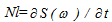 , is stabilized in the range ωo<ω/ωp<8, that provides a criterion for selecting the value of ωm. The choice ofω0 is justified only by the form of cutting factor M (ω, ωp) in (7).Following [12], for convenience in calculation of results, the magnitude of nonlinear energy transfer over any spectrum S(ω, θ), is defined as
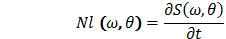 | (9) |
 | (10) |
 . It is the analysis of shape for function
  (which on angle-averaging is denoted as Nl(f)), arranged on the axis of the dimensionless frequency (ω/ωp), is of the primary interest here, regardless of quantitative values of the initial spectrum, peak frequency, and the nonlinear transfer.Note that this is the most effective way for comparing computational results obtained by using different calculating methods.
3. Numerical Results
- The results of calculations for the case of isotropic angular distribution of the spectra, obtained by two different methods of calculation for the KI [12, 13], are presented in Figs. 1 and 2. Regardless of the method of computing it is shown that for each of parameters, X = 4 and X = 11/3, the nonlinear transfer, Nl(f), substantially differs from the zero in the practically important frequency range, ω0<ω/ωp<6. These results give a clear and unambiguous conclusion about non-stationarity of spectra (4) and (5) on a limited frequency band, even in the case of an isotropic angular distribution of the spectra. Earlier in [12], it was shown that these spectra are also non-stationary for anisotropic angular distributions. (all results of our calculations are presented in detail on the site ArXiv.org [14]).
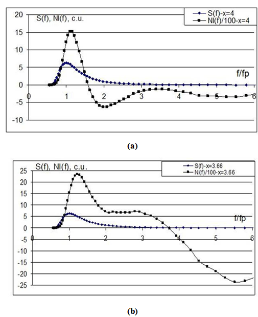 | Figure 1. One-dimensional spectrum (diamonds) and nonlinear transfer (triangles) for an angular isotropic spectrum calculated by algorithm [12]: a) X = 4; b) X = 11/3. Spectra and transfers are given in conventional units |
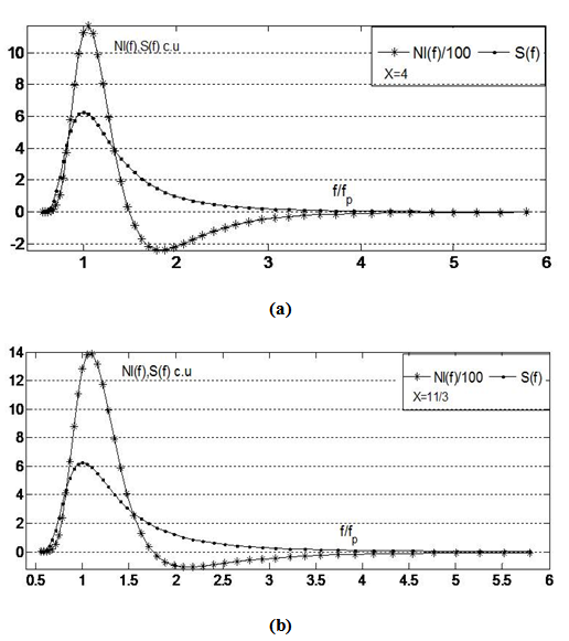 | Figure 2. Thesame as in Fig. 1, but by the WRT method [13]: a) X = 4; b) X = 11/3. Spectra and transfers are given in conventional units |
4. Analysis
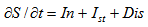
- In connection to the above discussions in Secs. 2 and 4, the question arises: whether the spectra of forms (4) and (5) can be found in nature, for example, in real wind waves. According to the theory and calculations [4, 7, 8, 9], the formation of Kolmogorov spectra in the framework of the GKE demands a fulfillment of the following three conditions:1) existence of the localized source, In, and sink, Dis, spaced on frequency band, to make the so-called "inertial range" [3]; 2) absence of sources and sinks (or negligible value of them compared with Nl), distributed within the inertial range; and 3) spectra must be averaged over a significant period of time (see Sec. 2). Let us make a brief analysis for feasibility of the above conditions in real wind waves.The modern understanding of mechanisms for the evolution of wind waves, in terms of the GKE [15], indicates that in the right hand side of equation (1), in addition to the term Ist. , there are two source terms: the wave energy input, In(ω,θ), and the sink, Dis(ω,θ), describing the dissipation of wave energy. However, the typical distribution of intensities of these terms, averaged over angle, (for example, taken from [15] and shown in Fig. 3) are far from the fulfillment of the above conditions: 1) and 2). Note that the explicit expressions for In and Dis are not critical here, due to the fact that their numerous versions differ insignificantly in quantity [15].
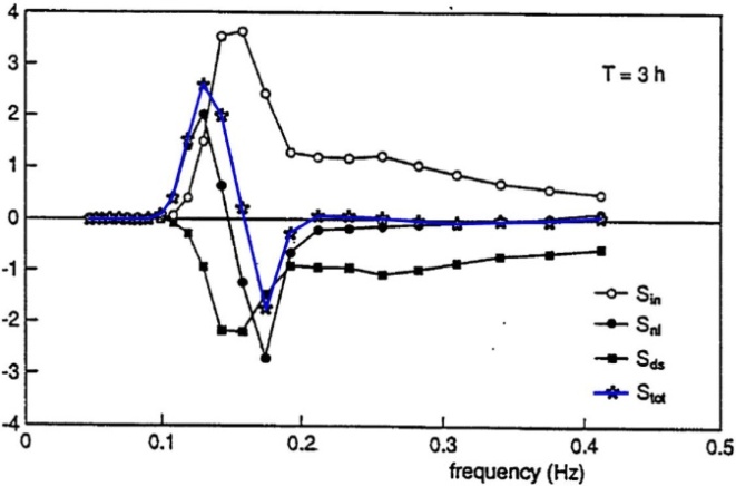 | Figure 3. Typical ratio of contributions from different mechanisms of evolution of wind involved in the generalized kinetic equation (model WAM) |
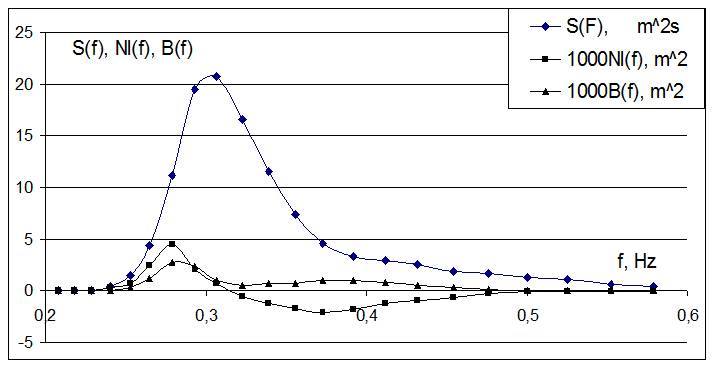 | Figure 4. Typical ratio of deposits terms Nl (f) and B (f) (in units. m2s) at a particular spectrum S (f) (in units. m2s) for developing waves (wind W = 10m / s) |
5. Discussion
- However, existence of the spectra with the tail of form (4) are often observed (e.g., [17-19]), the question arises about the nature of formation of such a spectra. Discarding the possibility of realization the constant nonlinear fluxes, PE or PN, due to the reasons said in Sec. 4, the only plausible justificating existence of the spectrum of form (4) can be obtained from the random-walk theory applied for vertical displacement of water surface in the phase-space. According to this theory, described by Golitsyn [3], it is sufficient to assume that the acceleration of the free surface,
 is affected by the random force of turbulent air pressure, having the white noise spectrum, P(ω). For a qualitative description of this process, it is necessary to represent the Euler equations for waves on liquid surface η(t) in a form of proper single equation., The final form of this equation in k-space has the kind
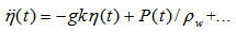 | (11) |
 means the random perturbations of the free surface due to turbulent air pressure at the interface, normalized by the water density, which provides the sought surface acceleration,
  . Therefore, if the perturbation has a frequency spectrum of the white noise, SP(ω)=const, , by assuming the other terms in the right-hand side of (11) to be relatively small, we get the same spectrum for the acceleration of liquid surface
  This implies immediately the spectrum elevations Sη(ω) of form (4) (for details, see [3]). Herewith, the dimension of coefficient in (4) is completely determined by the dimension of the disturbing force.In this regard, it is appropriate to recall Kitaigorodskii hypothesis[20], who obtained the spectrum with the tail of form (4) from the simplest dimensional considerations, taking three dimensional variables as a basis: frequency ω, friction wind speed u* and the acceleration of gravity, g. In such a case, the expression for the wind-wave frequency spectrum becomes,
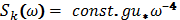 | (12) |
6. Conclusions
- In conclusion, it remains only to note that the spectra of form (10) are not always realized in the wind waves, even under stationary wind [21]. Apparently, some additional conditions are needed for realization the Kolmogorov-type spectra in wind waves, existence of which requires further investigations.
ACKNOWLEDGEMENTS
- The authors express their gratitude to Academician G.S. Golitsyn and Prof. P. F. Demchenko for a series of useful remarks expressed during the discussion of the paper.
Notes
- 1. For the first time it was derived by Hasselmann [5], and re-derived later by Zakharov [6]. The explicit form of the integrand is not principal here.2. It should be noted here that the distribution of balance B(f) can vary significantly, depending on the stage of wave development, characterized by the wave age, A, given by the ratio of the phase velocity for the dominant waves to the wind speed. Thus, wave age A may also affect the law of decay for the tail of the spectrum (see discussion in chapter 6.2 of book [3]).